Real-Time Evolution, Scattering, and Observable Extraction

A Hamiltonian regulator gives direct access to $U(t)=e^{-iHt}$ , but a finite-time signal is not automatically a continuum response or scattering amplitude. One must define the prepared state, physical sector, operator, time-evolution approximation, observation window, spatial boundaries, and asymptotic mapping. Each creates a distinct error axis that should be varied or bounded.

Required background. Regulated Hamiltonian field theory defines states and operators; retarded and spectral correlators define causal response.

Helpful background. Physical gauge Hilbert spaces control gauge sectors. LSZ reduction, relativistic kinematics, and cross sections supply the asymptotic scattering map.

Unequal-time and retarded response

Real-time observable card. Evolution uses a fixed regulated, self-adjoint Hamiltonian in continuous Lorentzian time. The prepared state, physical charge sector, operator renormalization, spatial boundaries, evolution tolerance, sampling cadence, and window $0\le t\le T$ are stated. The limits in time step, $T$ , packet width, $L$ , local dimension, and $a$ remain separate.

For a stationary state $\rho$ , the retarded correlator is

G_R(t,\mathbf x)=-i\theta(t) \operatorname{Tr}\!\left(\rho[O(t,\mathbf x),O(0)]\right), \qquad O(t)=e^{iHt}Oe^{-iHt}.

Its spectral density is $\rho_O(\omega,\mathbf p)=-2\operatorname{Im}G_R(\omega,\mathbf p)$ in a common convention. In finite volume the spectrum is discrete,

C(t)=\sum_n |\langle n\lvert O\rvert0\rangle|^2e^{-i(E_n-E_0)t}.

This finite-volume spectral sum is the regulated counterpart of the propagator spectral representation established by Lehmann 1954, pp. 342–357.

Multiplying by a window $w(t)$ before Fourier transformation convolves the true spectrum with $\widetilde w(\omega)$ . A duration $T$ gives resolution no better than order $2\pi/T$ , while late-time noise, reflections, or truncation error can force an earlier cutoff. Report the window and show stability under at least one alternative.

Controlled time evolution

If $H=A+B$ , a first-order product formula has

e^{-i(A+B)t}=\left(e^{-iA\delta t}e^{-iB\delta t}\right)^r +O(t\delta t\lVert[A,B]\rVert), \qquad r=t/\delta t,

whereas symmetric Strang splitting has global error $O(t\delta t^2)$ under suitable norm bounds. Many-body norms can make worst-case bounds loose, so refine $\delta t$ on the actual observables as well as checking unitarity.

Monitor energy, exact global charges, Gauss leakage, norm, and a held-out observable. Agreement of two algorithms at one step size is not a convergence study if their errors share the same commutator structure.

State preparation is another approximation. For an adiabatic path $H(s)$ , finite rate creates excitations governed by gaps and matrix elements; near criticality the gap can vanish with volume. Report overlaps, excess energy, symmetry quantum numbers, or independent correlators rather than assuming the named preparation protocol succeeded.

Wave-packet scattering at finite regulator

Prepare separated packets centered at momenta $\mathbf p_1,\mathbf p_2$ with width $\sigma_p$ . They must be narrow enough for a definite kinematic bin but localized enough to separate before collision:

a\ll \sigma_x\sim\sigma_p^{-1}\ll L, \qquad t_{\mathrm{collision}}+t_{\mathrm{separation}}<t_{\mathrm{wrap}}.

Evolve through the interaction and project onto outgoing packets or measure flux through a surface. Finite volume discretizes momenta, packet tails overlap, and periodic images eventually return. The extracted probability becomes a cross section only after flux normalization, phase-space conversion, stable-particle residue or operator matching, and appropriate $L\to\infty$ , packet, and continuum limits.

A complete scalar-field wave-packet construction, including preparation, evolution, and scattering extraction, is given by Jordan, Lee, and Preskill 2014, pp. 1014–1080.

Inclusive observables can sometimes be obtained from current response without reconstructing every exclusive final state. They still require a matched current, finite-time resolution model, and control of unobserved boundary flux.

The shared map locates all time-domain approximations after physical-sector construction.

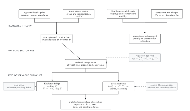
A regulated Hamiltonian and local Hilbert space feed exact constraints or penalty suppression, then a physical sector; a positive transfer-matrix branch and a direct real-time branch meet only at matched renormalized continuum observables, with leakage and positivity failures marked.

Direct real-time access avoids Euclidean analytic continuation, but it adds preparation, evolution-step, finite-window, and boundary controls. These remain separate from local-Hilbert and constraint errors upstream. The diagram is schematic.

A minimal error decomposition

Source	Diagnostic	Refinement
Preparation	energy variance, overlap, symmetry sector	slower path or improved ansatz
Evolution	norm, conserved charges, held-out observable	decrease $\delta t$ or algorithmic tolerance
Constraint	$\epsilon_G(t)$ or projector weight	exact basis/projector or penalty sequence
Time window	alternative tapers and endpoints	increase clean $T$
Boundary	reflected-front arrival and volume comparison	increase $L$ or absorb with quantified bias
Operator	Ward identity and matching factor	improve or nonperturbatively match
Field-theory target	$a$ , $d$ , basis, volume sequences	correlated continuum analysis

Adversarial failure case

Choose a window that extends just beyond the first periodic reflection and apply a taper that suppresses the visible time-domain echo. Two unitary algorithms can then conserve norm and energy and produce the same sharp Fourier peak, even though the peak contains wrapped flux rather than an asymptotic outgoing state. Increase $L$ at fixed physical packet and detector geometry, move the window endpoint across the predicted reflection time, and compare a local flux integral with packet projection. A physical pre-wrap signal is stable; the wrapped contribution moves with $L$ and the window.

Observable-level validation

Reproduce the exact small-system unequal-time correlator over the full fitted interval, not only at one endpoint.
Refine the evolution tolerance and confirm the predicted convergence order for the final response, flux, or packet probability.
Monitor energy, exact global charges, Gauss leakage, and one held-out observable throughout time.
Vary the window function, endpoint, sampling cadence, spatial volume, and detector surface independently.
Close the normalization from the prepared-state overlap and incident flux through the final phase-space or spectral conversion.

Common pitfalls

Equating a Fourier peak with a stable particle. Finite-window side lobes and multiparticle levels can mimic peaks. Vary the window, volume, and interpolating operator.

Extrapolating step size at one time only. Errors can grow with $t$ and change phase. Test the full time interval used in extraction.

Calling packet counts a cross section. Convert through incident flux, final-state measure, residue conventions, and asymptotic limits.

Learning outcomes

Specify a finite-volume, finite-time protocol for a retarded, spectral, inclusive, or wave-packet observable and compute the normalization that maps its estimator toward the intended continuum quantity.
Given two agreeing time evolutions, design step-size, window, boundary, preparation, and constraint tests that can falsify a shared real-time artifact.

Exercises

A clean signal lasts to $T=50/m$ . Estimate its Fourier-bin scale.

Solution

$\Delta\omega\sim2\pi/T\simeq0.126m$ . Window choice can broaden it further.

Why can exact norm conservation coexist with Gauss-law violation?

References

Section titled “References”- Jordan, S. P., Lee, K. S. M., and Preskill, J. (2014). Quantum algorithms for quantum field theories. Quantum Information and Computation, 14, 1014–1080. arXiv.
- Lehmann, H. (1954). On the properties of propagation functions and renormalization constants of quantized fields. Il Nuovo Cimento, 11, 342–357. DOI.
Further reading
Section titled “Further reading”- Källén, G. (1952). On the definition of the renormalization constants in quantum electrodynamics. Helvetica Physica Acta, 25, 417–434. Persistent record.