Hilbert-Space Truncation as a Regulator

A Hilbert-space projector is a controlled regulator when its retained and omitted subspaces are defined without ambiguity, the sequence approaches a dense domain appropriate to the target Hamiltonian, omitted-state effects are represented or bounded, and all other limits are kept identifiable. Projecting $H$ to a finite matrix without these conditions is an approximation whose error need not vanish, need not be monotone, and need not be shared by other observables.

Required background. Regulated Hamiltonian Field Theory supplies the self-adjoint regulated Hamiltonian and its continuum target. Normal Forms, Spectra, and Projectors supplies spectral projectors, invariant subspaces, and the min–max principle.

Helpful background. QFT Regulator Families and Their Tradeoffs supplies the distinction between a regulator definition and regulator removal.

A truncation is a sequence of projectors

Projector and limit contract. Declare the target regulated Hamiltonian $H$, its domain and exact symmetries; the orthogonal projector $P_\Lambda$; the omitted projector $Q_\Lambda=1-P_\Lambda$; every cutoff and volume; the counterterms and effective operators included at that cutoff; and the order or joint strategy for all limits. The label $\Lambda$ may be an energy, particle number, mode, representation, or local-state cutoff, but its numerical value and physical units must be explicit.

For a cutoff family to approximate the full Hilbert space, one normally asks for strong convergence

$$P_\Lambda|\psi\rangle\longrightarrow|\psi\rangle \quad\text{as}\quad \Lambda\to\infty$$

on a dense set. That condition alone is not enough for an unbounded Hamiltonian: the projected quadratic forms must also approximate the form of $H$ on its form domain. Under the usual self-adjointness, lower-bound, and compactness hypotheses, nested Rayleigh–Ritz spaces then converge to isolated discrete eigenvalues according to the min–max principle Reed and Simon 1978, Chapter XIII, §1.

Common choices remove different physics:

• Free-energy cutoff: retain $H_0$ eigenstates with $E_i^{(0)}\le E_{\max}$. It is natural for weak or relevant deformations but treats interacting high-energy eigenstates only indirectly.
• Particle-number cutoff: retain at most $N_{\max}$ quanta. It can remove low-energy many-particle states and therefore is not purely ultraviolet.
• Mode or momentum cutoff: retain specified Fourier modes. It is ultraviolet in momentum, but occupation numbers may still make the space infinite.
• Representation cutoff: retain irreducible representations below a Casimir or highest-weight bound. Gauge and global constraints can remain exact, while virtual representations induce new interactions.
• Local-state cutoff: retain finitely many states per site. It is useful for bosons and tensor networks, but a growing lattice volume magnifies each local omission.

Two schemes with the same matrix dimension are not equivalent regulators. Their $Q_\Lambda$ spaces differ, so their induced operators and asymptotic errors differ.

Omitted states induce an exact energy-dependent interaction

Let $H|\Psi\rangle=E|\Psi\rangle$ and write $|\psi_P\rangle=P|\Psi\rangle$, $|\psi_Q\rangle=Q|\Psi\rangle$. The block equations are

$$PHP|\psi_P\rangle+PHQ|\psi_Q\rangle=E|\psi_P\rangle,$$ $$QHP|\psi_P\rangle+QHQ|\psi_Q\rangle=E|\psi_Q\rangle.$$

If $E-QHQ$ is invertible on the omitted subspace, the second equation gives

$$|\psi_Q\rangle=(E-QHQ)^{-1}QHP|\psi_P\rangle.$$

Substitution yields the exact Feshbach–Schur operator

$$H_{\mathrm{eff}}(E) =PHP+PHQ(E-QHQ)^{-1}QHP.$$

The second term is what a bare projection drops. It contains virtual paths that leave the retained space and return. Its expansion may generate vacuum energy, masses, couplings, derivative operators, nonlocal terms, and state-dependent corrections. Feshbach’s projection formalism provides this exact reduction Feshbach 1958, §§ 2–3; its systematic use in Hamiltonian truncation is developed in Elias Miró and Ingoldby 2023, §§ 2–4.

Exactly checkable two-state benchmark

Take

$$H=\begin{pmatrix}0&g\\ g&\Delta\end{pmatrix}, \qquad P=\begin{pmatrix}1&0\\0&0\end{pmatrix}, \qquad \Delta>0.$$

The projected Hamiltonian $PHP$ predicts $E=0$. Exact elimination instead gives

$$E=\frac{g^2}{E-\Delta},$$

whose lower solution is

$$E_-=\frac{\Delta-\sqrt{\Delta^2+4g^2}}{2} =-\frac{g^2}{\Delta}+\frac{g^4}{\Delta^3} +O\!\left(\frac{g^6}{\Delta^5}\right).$$

This one-line benchmark detects a wrong resolvent sign, a missing second-order shift, and an expansion used outside $|g/\Delta|\ll1$. It also demonstrates that an omitted state can affect a low eigenvalue even when its bare energy is large.

Variational monotonicity has precise hypotheses

Let $V_1\subset V_2\subset\cdots$ be nested finite-dimensional subspaces of the quadratic-form domain of a self-adjoint $H$ bounded below. For discrete eigenvalues below the essential spectrum, the $k$th Ritz value obeys

$$E_k^{(n+1)}\le E_k^{(n)}, \qquad E_k\le E_k^{(n)}.$$

For $k=0$, this follows immediately because minimizing the Rayleigh quotient over a larger set cannot raise its infimum. For excited states it follows from the min–max characterization, provided the ordered level is tracked in the same exact symmetry sector. The statement can fail to be useful when spaces are not nested, the Hamiltonian or fitted parameters change with $n$, a level crosses another sector, the basis metric is mishandled, or the target lies in a continuum.

Even when the theorem applies, it does not imply monotonic convergence of $E_1-E_0$, $\langle O\rangle$, a transition amplitude, or a real-time signal. Both energies in a gap are upper bounds, so their difference has no fixed sign of error.

Ultraviolet, infrared, and limit order remain separate

For a scalar field of mass $m>0$ on a circle,

$$H_0=\sum_{n\in\mathbb Z}\omega_n a_n^\dagger a_n, \qquad \omega_n=\sqrt{m^2+(2\pi n/L)^2},$$

the free-energy projector is

$$P_{E_{\max}}= \sum_{\{N_n\}:\,\sum_n\omega_nN_n\le E_{\max}} |\{N_n\}\rangle\langle\{N_n\}|.$$

At fixed $L$ this makes each momentum and $\mathbb Z_2$ sector finite. Raising $E_{\max}$ restores omitted virtual states; raising $L$ changes momentum spacing and physical finite-volume effects. A sequence with $E_{\max}\propto L$ can conceal cancellation between the two. The calculation must either take a justified order of limits or sample enough of the $(E_{\max},L)$ plane to estimate cross terms.

The same warning applies to a spatial lattice spacing $a$, local occupation $n_{\max}$, basis scale $\mu$, and particle cutoff $N_{\max}$. A truncation study that varies only a composite cost label cannot assign a continuum uncertainty to its individual sources.

The convergence map closes the omitted-state loop

Read the following schematic from the $P/Q$ split to the held-out branch. The solid path records a controlled construction; the dashed branch is a false plateau that must trigger a revision rather than a smaller quoted error.

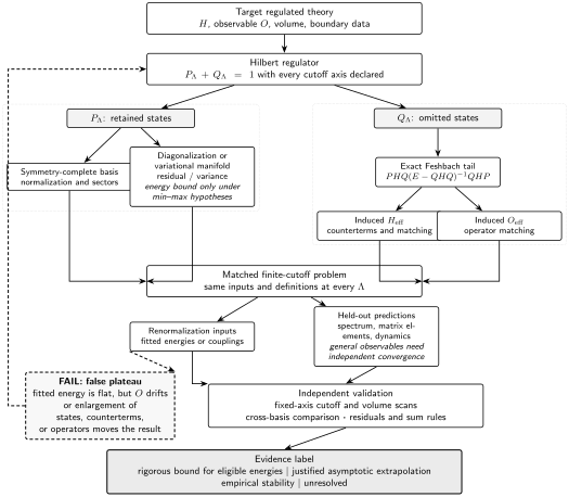
A Hilbert-space cutoff is controlled only when omitted states feed the effective Hamiltonian and observables and when independent cutoff, basis, volume, residual, and held-out tests close the loop. Monotone variational energy bounds are distinguished from general observable convergence; the dashed false-plateau branch is schematic and not to scale.

Minimum truncation certification record

The same semantic record accompanies every method in this chapter so that a claim cannot silently lose its omitted-state or observable assumptions.

Required fields for a truncation result and the test that can falsify each field.

Field	Required declaration	Independent test	Failure signal
Target	Hamiltonian, prior regulator, volume, boundary data, observable	Units and free or exact limit	Changing target across cutoff points
Projectors	PΛ, QΛ, all cutoff axes, limit order	State counts and nestedness	Unidentified omitted states
Basis and sectors	Normalization, Gram matrix, null removal, exact charges	Hermiticity and selection rules	Duplicates or broken constraints
Induced Hamiltonian	Derived operator basis and approximation order	Omitted-state toy model or perturbative coefficient	Drift incompatible with the declared tail
Counterterms	Inputs, running coefficients, and no-double-counting rule	Refit protocol at every cutoff	A fitted datum presented as a prediction
Variational status	Manifold, optimizer, symmetry, bound hypotheses	Residual, variance, and ansatz enlargement	Energy plateau with a large residual
Effective observables	Projected and induced operator terms	Sum rule or matched matrix element	Spectrum stable while the observable drifts
Cutoff sequence	Independent basis, volume, counterterm, time, and state scans	Fixed-axis and cross-term fits	Only one diagonal sequence
Extrapolation	Asymptotic form, fit window, covariance, alternatives	Window and model stability	Exponent chosen from the desired answer
Held-out tests	Unused spectrum, matrix element, dynamics, and second basis	Blind comparison after choices freeze	All tests participated in tuning
Adversarial enlargement	Larger state and operator bases	Repeat the full match and prediction	Former plateau moves beyond its error
Claim	Bound, asymptotic evidence, empirical stability, or unresolved	Error and cost reproduced independently	Precision exceeds the weakest test

Adversarial failure: a particle cutoff that never becomes complete

Suppose an interacting theory is computed at $N_{\max}=2,3,4$ while the momentum grid is also refined, and a mass appears stable. If the sequence then keeps $N_{\max}=4$ while only the momentum grid continues to improve, it does not approach the full Fock space. Multi-particle virtual contributions remain in $Q$, and their effect may not be absorbable by the chosen mass counterterm. The smooth mass curve establishes a limit of the four-particle model, not of the target QFT.

The remedy is to state the fixed-$N_{\max}$ theory as its own approximation, increase particle number on a separate axis, include the induced operators required by omitted sectors, and test an observable sensitive to those sectors. A failure to afford that scan remains an explicit systematic error.

Observable-level validation checklist

• Verify $P_\Lambda^2=P_\Lambda$, $P_\Lambda^\dagger=P_\Lambda$, and $[P_\Lambda,G]=0$ for every symmetry generator claimed exact.
• Compare enumerated state counts against an independent small-cutoff construction and check that the union of retained spaces is dense in the declared domain.
• Reproduce the two-state energy and resolvent sign above before using an omitted-state expansion.
• Separate ultraviolet, volume, particle, mode, representation, local-state, basis-scale, and optimization axes.
• Track eigenpair residuals and variances, but do not equate them with truncation error.
• Reserve an unfitted matrix element or sum rule and repeat it after enlarging both the state and effective-operator bases.
• State whether an energy is a rigorous Ritz bound, an extrapolation, an empirically stable value, or an unresolved finite-cutoff estimate.

You should now be able to (1) write a projector definition that exposes retained states, omitted states, exact sectors, scales, and limit order, and (2) decide from the min–max hypotheses whether a convergence statement is a rigorous energy bound or only empirical evidence. Basis Construction, Symmetry Sectors, and Matrix Elements turns the projector into a checked matrix; Renormalizing a Truncated Hamiltonian approximates the exact omitted-state term. Local-Hilbert and gauge-basis regulators originate in Hamiltonian Lattice Field Theory.

Exercises

Recover the exact two-state energy

Starting from $H_{\mathrm{eff}}(E)$ for the two-state matrix above, derive both eigenvalues and identify which branch has a regular expansion near $g=0$ and $E=0$.

Solution

Here $PHP=0$, $PHQ=g$, and $QHQ=\Delta$, so $H_{\mathrm{eff}}(E)=g^2/(E-\Delta)$. The equation $E=g^2/(E-\Delta)$ gives

$$E^2-\Delta E-g^2=0, \qquad E_\pm=\frac{\Delta\pm\sqrt{\Delta^2+4g^2}}2.$$

The minus branch approaches $0$ and expands as $-g^2/\Delta+g^4/\Delta^3+\cdots$. The plus branch approaches the omitted bare level $\Delta$; it is not represented by a low-energy effective Hamiltonian expanded about $E=0$.

Test a proposed nested sequence

For a scalar circle basis, scheme A keeps all states with $E^{(0)}\le 10,12,14$, while scheme B keeps the lowest $100,150,200$ states separately in each interacting symmetry sector after diagonalizing a preliminary Hamiltonian. Which sequence supports direct Rayleigh–Ritz monotonicity, and what must be checked for the other?

Solution

Scheme A is nested if the same $H_0$, volume, boundary conditions, and exact sector definitions are used at every cutoff. Its ordered Ritz energies then obey the min–max inequalities under the stated domain hypotheses. Scheme B is not automatically nested: the preliminary eigenvectors and even the selected subspace may change at every step. One must explicitly test $V_n\subset V_{n+1}$ or abandon the monotonic-bound claim. Both schemes still need effective-observable and held-out tests.

References

• Elias Miró, Joan, and James Ingoldby. “Effective Hamiltonians and Counterterms for Hamiltonian Truncation.” Journal of High Energy Physics 2023, 052 (2023). DOI. Open PDF.
• Feshbach, Herman. “Unified Theory of Nuclear Reactions.” Annals of Physics 5, no. 4 (1958): 357–390. DOI.
• Reed, Michael, and Barry Simon. Methods of Modern Mathematical Physics IV: Analysis of Operators. Academic Press, 1978. Publisher record.