Correlated Fits, Model Selection, and Stability Tests

A lattice fit usually acts on a highly correlated vector whose covariance is itself estimated. A convincing parameter estimate therefore needs more than a plausible curve and acceptable $\chi^2$: the model must be identifiable on the chosen window, covariance treatment must be stable and calibrated, residuals must be structured as expected, and competing descriptions must be tested on synthetic or held-out data.

Required background. Estimators, covariance, and resampling define the joint data uncertainty; operator bases and excited states define the spectral models.

Helpful background. Continuum extrapolation shows the same correlated-fit principles across ensembles.

Correlated objectives

Local fit convention and regime. The fitted vector, time or ensemble window, covariance estimator, effective number of independent blocks, model family, and any priors are fixed as one procedure. $C$ is the covariance of the estimated data vector, not of individual raw measurements, and every synthetic or resampled repetition re-estimates and regularizes it exactly as production does. Reported intervals cover the complete declared selection procedure, not only a fit conditional on the chosen model and window.

For data vector $\mathbf y$, model $\mathbf f(\boldsymbol\theta)$, and covariance $C$, the Gaussian objective is

$$\chi^2(\boldsymbol\theta)= [\mathbf y-\mathbf f(\boldsymbol\theta)]^T C^{-1}[\mathbf y-\mathbf f(\boldsymbol\theta)].$$

This form is appropriate only when the estimated mean is sufficiently Gaussian and the covariance procedure is part of the calibration. If $C$ is estimated from the same finite sample, the nominal $\chi^2$ distribution is altered. Resampling or synthetic repetitions should include covariance re-estimation; Michael 1994, pp. 2616–2619 treats the finite-sample correlated-fit issue in a lattice setting.

Whitened residuals

$$\mathbf r_w=C^{-1/2}[\mathbf y-\mathbf f(\widehat{\boldsymbol\theta})]$$

should show no systematic time, momentum, or ensemble structure. A small total $\chi^2$ can coexist with coherent residuals when covariance eigenmodes are poorly estimated or overregularized.

Spectral-window example

Consider

$$C(t)=A_0e^{-E_0t}+A_1e^{-E_1t}+\cdots.$$

A one-state fit at late time reduces excited-state bias but loses signal; a two-state fit at earlier time adds weakly identified parameters. Vary $t_{\min}$ and $t_{\max}$, operator basis, and model order. Inspect parameter correlations and the singular values of the model Jacobian

$$J_{ti}=\frac{\partial f_t}{\partial\theta_i}.$$

If a direction of $J^TC^{-1}J$ is nearly null, the data do not identify that parameter without a prior or external constraint. A stable $E_0$ caused by a strong prior is prior-conditioned evidence and should be labeled as such; Lepage et al. 2002, pp. 12–20 gives the constrained-fitting framework rather than a license to erase prior sensitivity.

Synthetic closure should draw correlated two-state data with known parameters, rerun the complete window and model-selection procedure, and measure bias and interval coverage. A plateau-only adversary with an unresolved second state is particularly important.

Covariance regularization

If $C=V\operatorname{diag}(\lambda_i)V^T$ is noisy, hard singular-value cuts replace $C^{-1}$ by a pseudoinverse on retained modes; shrinkage uses

$$C_\alpha=(1-\alpha)C+\alpha T$$

for a declared target $T$. Both alter weights and goodness-of-fit calibration. Vary the cutoff or shrinkage strength, show which residual modes are removed, and repeat coverage tests. Choosing the setting that minimizes the final error is an analysis choice, not validation.

Model comparison and averaging

Information criteria, marginal likelihoods, cross-validation, or predeclared fit-quality rules compare models under different assumptions. None proves that the candidate set contains the truth. Akaike’s information-criterion construction is derived in Akaike 1974, pp. 716–723. If estimates $\widehat\theta_m$ are combined with weights $w_m$, a useful variance decomposition is

$$\operatorname{var}(\theta)= \sum_mw_m\left[\operatorname{var}_m(\theta) +(\widehat\theta_m-\overline\theta)^2\right], \qquad \overline\theta=\sum_mw_m\widehat\theta_m.$$

State whether $w_m$ are fixed, data dependent, Bayesian, or heuristic, and calibrate the complete selection or averaging procedure. Treating the spread of only accepted models as a frequentist confidence interval has no automatic coverage guarantee.

The graph places model choices upstream of scale, matching, and continuum fits, so their covariance and alternatives must propagate.

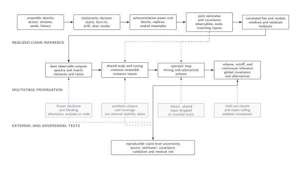
Correlated fitting is one node in a larger dependency graph. Window, covariance, and model alternatives must be repeated through scale, renormalization, and continuum stages rather than appended as an uncorrelated percentage. The diagram is schematic.

Stability tests that answer different questions

Variation	Diagnoses	Does not prove
Move fit window	contamination and signal loss	completeness of model set
Change operator basis	overlap and rank sensitivity	absence of all missing states
Vary covariance conditioning	noisy eigenmode dependence	correct likelihood calibration
Add/remove state or cutoff term	model-order sensitivity	that the larger model is identifiable
Hold out times or ensembles	local predictive adequacy	continuum universality
Synthetic closure	bias and coverage under fixture	correctness outside fixture family

Adversarial failure: a discarded covariance mode carries the discrepancy

Take a trusted positive-definite fixture with eigenpair $(\lambda_{\min},\mathbf v_{\min})$ and inject

$$\delta\mathbf y=5\sqrt{\lambda_{\min}}\,\mathbf v_{\min}$$

relative to the fitted model. With the full covariance, this one direction contributes $\delta\chi^2=25$. A hard singular-value cut that discards $\mathbf v_{\min}$ assigns it zero weight and can turn the same visibly constrained discrepancy into an acceptable reported fit. The production test must expose the removed mode, repeat the complete cut rule on synthetic data, and fail if nominal intervals lose coverage or the target shifts materially as that mode is restored.

Observable-level validation checklist

• Record the complete data vector, fit window, covariance source, conditioning rule, candidate models, priors, and selection rule before interpreting the target parameter.
• Inspect whitened residuals by time, momentum, channel, and ensemble rather than relying on a scalar $\chi^2$.
• Diagnose identifiability with parameter correlations and singular values of $J^TC^{-1}J$; vary any influential prior.
• Track every removed or shrunk covariance eigenmode and repeat goodness-of-fit calibration after covariance re-estimation.
• Run the full window, conditioning, and model-selection procedure on synthetic correlators and measure bias plus interval coverage.
• Inject the five-sigma covariance-mode adversary above and require the stability report to reveal its effect.
• Hold out at least one informative time range, channel, or ensemble when the data volume permits, and state what that prediction does not test.

Common pitfalls

Using visual smoothness as fit validation. Strong correlations make many points move together; a curve can look excellent while missing a constrained eigenmode.

Selecting a window after viewing the desired value. Freeze the rule, blind the target, or propagate the selection procedure through alternatives.

Reporting only the preferred model. Show the plausible set, weights or acceptance rule, and the between-model component.

Learning outcomes

1. Fit a correlated synthetic correlator with at least two plausible spectral models and quantify parameter, window, covariance-conditioning, and prior sensitivity with bias and coverage results.
2. Given a smooth-looking fit or discarded-mode adversary, decide whether the target is identifiable and report a model-dependent interval without treating visual stability or nominal goodness of fit as proof of adequacy.

Exercises

1. Why can dropping a small covariance eigenvalue reduce $\chi^2$ dramatically?

Solution

The inverse weights residuals by $1/\lambda_i$. A small eigenvalue gives a large penalty to its residual direction; dropping it removes that constraint entirely, whether it was noisy or informative.

2. What does a successful two-exponential synthetic closure fail to establish?

Solution

It establishes behavior for the tested noise, covariance, amplitudes, gaps, and candidate models. It does not cover oscillating states, continuum spectra, different gaps, non-Gaussian tails, or other omitted structures.

References

• Akaike, H. (1974). A new look at the statistical model identification. IEEE Transactions on Automatic Control, 19, 716–723. DOI.
• Lepage, G. P. et al. (2002). Constrained curve fitting. Nuclear Physics B Proceedings Supplements, 106–107, 12–20. DOI.
• Michael, C. (1994). Fitting correlated data. Physical Review D, 49, 2616–2619. DOI.