

Euclidean Correlators and Spectral Information
Euclidean lattice two-point functions encode discrete finite-volume energies through exponential transfer-time dependence and operator overlaps through their coefficients. The measured correlator is the primary quantity; an energy, effective-energy plateau, or spectral peak is inferred from it under a model. Boundary images, thermal transitions, contact terms, operator normalization, covariance, and the noise floor must be separated before that inference begins.
Required background. Lattice Momentum, Propagators, and Cutoff Dispersion fixes finite Fourier and transfer-energy normalization. Euclidean Correlators and Schwinger Functions distinguishes Euclidean correlation functions from Lorentzian ordered correlators.
Helpful background. Spectral Decomposition of Two-Point Functions supplies the continuum state-insertion argument.
In the chapter’s observable-chain table, this page supplies the correlator and state-isolation data that every later matrix-element or spectral claim inherits.
From a lattice operator to a spectral sum
Section titled “From a lattice operator to a spectral sum”Let be operators on a time slice, projected onto a definite lattice momentum and exact lattice quantum numbers. With a positive transfer operator and temporal extent ,
For reflection-positive Wilson lattice gauge theory, a self-adjoint, strictly positive transfer matrix can be constructed explicitly Lüscher 1977, pp. 283–292. In other discretizations, positivity and the existence of the transfer description are assumptions to verify rather than automatic properties.
Inserting finite-volume energy eigenstates gives the exact thermal sum
When , vacuum propagation dominates the outer trace. For a zero-vacuum-expectation operator,
where ,
This page uses unit-normalized finite-volume states. With relativistic normalization, completeness inserts the appropriate inverse state-normalization factor; any redefinition that absorbs its square root into an overlap must also be used when defining three-point matrix elements.
For a self-adjoint or suitably self-conjugate basis, reflection relates to and a diagonal one-state correlator becomes a cosh. For charged or otherwise non-self-conjugate operators, backward propagation is an antiparticle or reversed-channel contribution and can have different overlaps. The exact thermal double sum above remains valid in either case.
Correlator conventions. This page uses Euclidean transfer time, periodic bosonic temporal boundaries, unit-normalized finite-volume states, zero-temperature language only when thermal terms are demonstrably suppressed, and the site-wide conventions. Operators are momentum projected with declared spatial-volume factors. Vacuum subtraction, reflection parity, smearing, and any conversion to another state normalization are local data.
For a Hermitian operator in a reflection-positive theory, diagonal spectral weights are nonnegative. Off-diagonal matrix elements can have either sign or phase. The matrix satisfies under the usual conjugation, and at fixed positive time it is positive semidefinite for suitable operator combinations. Violations beyond uncertainty flag normalization, conjugation, sampling, or positivity problems before fitting.
Effective energies are diagnostics, not states
Section titled “Effective energies are diagnostics, not states”For one correlator and lattice spacing , define
when the backward image is negligible. In a strict two-state truncation, gives
The approach to a plateau depends on the overlap ratio , not only on the energy gap. A small overlap can produce an early plateau; opposite-sign contributions in non-positive or subtracted channels can produce a false one.
Near the temporal midpoint, use the periodic one-state relation
instead of an infinite-time logarithmic ratio. Failure of neighboring time slices to yield a consistent cosh energy is a boundary-image diagnostic, not permission to discard them selectively.
The correlator-to-inference diagram shows which derived object is introduced at each stage. Inspect especially the branch from raw correlation data to fit assumptions and the distinction between a fitted spectral parameter and a renormalized target observable.
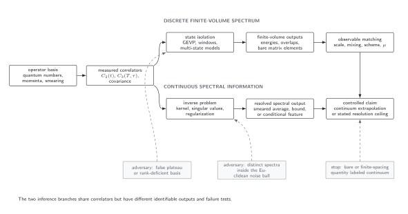
Two inference problems share the same regulated correlators. Discrete energies and overlaps, together with validated connected and disconnected three-point estimators, support bare matrix elements that require matching and continuum control before becoming physical results. Continuous reconstruction identifies only smeared averages, bounds, or conditional features at the demonstrated resolution; without separate matching and continuum analysis it ends at a methodological ceiling. Dashed boxes mark failure tests. The diagram is schematic and not to scale.
Exact free-scalar benchmark
Section titled “Exact free-scalar benchmark”For the nearest-neighbor free scalar at fixed spatial momentum, the infinite-time correlator is
with given by the exact lattice dispersion. At finite periodic ,
This fixture tests four pieces independently: the pole energy, residue, backward image, and temporal periodicity. A fitter that recovers the energy but not the exact amplitude has not passed the normalization check. A model that omits the image should fail when the fit window approaches .
The periodic expression follows by summing images of the infinite-time Green function:
The prefactor is the residue obtained by solving the nearest-neighbor temporal difference equation, or equivalently by evaluating the pole of its discrete Fourier representation. The image sum then checks the finite-period formula independently of a fitting routine.
The QFT.org 2026 Chapter 2 benchmark, validated snapshot evaluates the same correlator both as a discrete Fourier sum and in closed form. For , , and the declared spatial-frequency fixture, the two routes agree within , the input lattice energy is , and the exact-midpoint one-sided estimator is . It also checks that the one-sided estimator changes sign at the half-step straddling the midpoint, whereas the three-point cosh estimator returns the input energy.
Signal, variance, and the usable window
Section titled “Signal, variance, and the usable window”Statistical precision usually worsens with Euclidean time because the variance is itself a correlation function with its own lightest allowed state. If the signal behaves as and its standard deviation as , then
The exponent is channel dependent. For baryons in QCD the classic signal-to-noise analysis relates the signal to the baryon mass and the variance to multi-pion states Parisi 1984, pp. 203–211. The general lesson is not a universal exponent: late time can reduce excited-state bias while increasing variance and covariance ill-conditioning.
A valid analysis window must therefore lie between two failures:
- too early, where omitted states or contact terms matter;
- too late, where the data no longer distinguish the model or thermal images matter.
Window choice is a model decision. It belongs in stability tests and uncertainty propagation, not in an undocumented visual selection.
Failure modes and checks
Section titled “Failure modes and checks”Vacuum subtraction omitted. If , the correlator contains a constant disconnected term. Subtract it with its covariance or include it in the model.
Finite-temperature terms called excited states. Thermal transitions depend on both and and can involve pairs of nonvacuum states. Varying distinguishes them from ordinary vacuum excitations.
Operator normalization changes across ensembles. Smearing radius, momentum projection, or field normalization can change overlaps even when energies agree. Record the transformation and avoid interpreting raw amplitudes across unmatched definitions.
Correlated data fitted as independent. Neighboring times and matrix elements often share configurations. A visually good fit can have invalid uncertainty when covariance is ignored.
Noise floor mistaken for a plateau. When the likelihood is insensitive to the energy, stable central values can reflect priors or parameter bounds. Inspect profile likelihoods or posterior-prior comparison and mock-data coverage.
Observable-level validation checklist
Section titled “Observable-level validation checklist”Before inferring spectral parameters, verify:
- operator quantum numbers, momentum projection, normalization, and smearing are fixed;
- vacuum, contact, boundary-image, and thermal terms are either modeled or bounded;
- and applicable positivity tests hold;
- an exact free or synthetic correlator is recovered with the same code path;
- covariance estimation and regularization are declared;
- early- and late-time stop conditions are quantified;
- multiple windows and state counts are compared; and
- measured correlators, fitted parameters, and renormalized observables are reported as distinct objects.
Exercises
Section titled “Exercises”1. Thermal image bias on a discrete grid. For , compute the one-sided logarithmic effective energy. Find its zero and its value at an exact midpoint lattice site. Explain why the cosh estimator behaves differently.
Solution
Write and
Then
It vanishes at , or : the zero lies halfway between the two correlator samples being compared. If is odd this is a lattice site. If is even, the estimator changes sign across the midpoint without vanishing on a site, and at the exact midpoint
not zero. This tends to zero only in the continuum-time limit at fixed . By contrast, substituting the one-state correlator into gives at every time, so the cosh estimator returns exactly.
2. Positivity of a correlator matrix. Show from the spectral sum that for when the weights are vacuum matrix elements in a positive Hilbert space.
Solution
Contracting gives
A negative eigenvalue larger than uncertainty therefore contradicts at least one assumption entering the declared matrix.
What you can now do
Section titled “What you can now do”You should now be able to derive a normalized finite-volume spectral sum and distinguish energies, overlaps, thermal images, effective-energy diagnostics, and noise limits before choosing a fit model. Continue with Operator Bases, Effective Masses, and Excited-State Control to determine which levels a correlator matrix can actually resolve.
References
Section titled “References”- Lüscher, Martin. “Construction of a Selfadjoint, Strictly Positive Transfer Matrix for Euclidean Lattice Gauge Theories.” Communications in Mathematical Physics 54, no. 3 (1977): 283–292. doi:10.1007/BF01614090.
- Parisi, Giorgio. “The Strategy for Computing the Hadronic Mass Spectrum.” Physics Reports 103, nos. 1–4 (1984): 203–211. doi:10.1016/0370-1573(84)90081-4.
- QFT.org. “Lattice Observables and Continuum Inference Benchmark.” JavaScript source, validated 25 August 2026. SHA-256
d76924d8c724cb7c9307fb38265336495fa3ff1a98103b3fa4fa734262647c2a. Reproducibility record.
Further reading
Section titled “Further reading”- Gattringer, Christof, and Christian B. Lang. Quantum Chromodynamics on the Lattice: An Introductory Presentation. Springer, 2010, ch. 5. doi:10.1007/978-3-642-01850-3.
- Michael, Christopher. “Adjoint Sources in Lattice Gauge Theory.” Nuclear Physics B 259, no. 1 (1985): 58–76. doi:10.1016/0550-3213(85)90297-4.
- Rothe, Heinz J. Lattice Gauge Theories: An Introduction. 4th ed. World Scientific, 2012, ch. 10. doi:10.1142/8229.