

Scattering Amplitudes and Resonance Poles from Finite-Volume Spectra
Finite-volume levels constrain an elastic amplitude only on the real axis. A resonance pole is obtained in a second step: fit the correlated levels with unitary real-axis parametrizations, reproduce the spectrum through the same quantization condition, then analytically continue each acceptable amplitude along a named path to a named sheet. A pole supported only by one fit form, partial-wave truncation, or threshold convention is model information, not a finite-volume observation.
Required background. Elastic Two-Body Quantization Conditions supplies the spectrum map and branch choice. Moving Frames, Cubic Irreducible Representations, and Partial-Wave Mixing supplies the finite-volume blocks. Resonance Poles, Riemann Sheets, and Unstable States supplies the infinite-volume pole and sheet definitions.
Helpful background. Correlated Fits, Model Selection, and Stability Tests supplies likelihood and alternative-model controls.
A unitary real-axis amplitude
Section titled “A unitary real-axis amplitude”For one elastic partial wave, define
on the upper physical bank. Then is real for real inside the elastic interval and , so unitarity is exact for every real fit parameter. This differs by a displayed phase-space factor from the dimensionless used on Partial-Wave Unitarity; the invariant check is the same and the same pole.
Amplitude and continuation convention. The fitted object is a unitary real-axis amplitude in the stated elastic interval; any pole claim also fixes the momentum branch, crossed cut, destination sheet, and residue normalization.
The detailed choices are:
| Field | Choice used on this page |
|---|---|
| Data likelihood | The primary data vector is the complete set of fitted finite-volume energies; its covariance includes common masses, anisotropy, and scale inputs |
| Real-axis amplitude | on the upper physical bank; is real in the fitted elastic interval |
| Threshold branch | immediately above threshold on the upper bank; the continuation path, crossed cut, and resulting sheet are stated |
| Pole convention | locally, and with |
| Fit alternatives | At least two unitary forms and the lowest allowed omitted partial wave are propagated |
| Supported conclusion | Finite-volume data directly support real energies; amplitudes require the quantization hypotheses, and poles additionally require analytic continuation |
Two useful elastic families are:
and a pole-plus-background matrix,
The first is a threshold expansion whose radius is limited by the nearest left-hand or inelastic singularity. The second is a real-axis parametrization; is not automatically the resonance pole mass. Truncating either family is a model choice even though elastic unitarity is exact.
Fit levels, not converted points
Section titled “Fit levels, not converted points”Let the measured spectrum be with covariance . For parameters , solve each irrep quantization condition for and minimize
Root identities must be tracked continuously. Sorting roots by energy can switch levels at an avoided crossing and make the objective discontinuous; match them by irrep, operator-overlap information, and continuity from a known parameter point.
Converted values of are excellent diagnostics but a poor default likelihood. The conversion is nonlinear, branches can jump, and common masses make points from different levels correlated. Fitting energies retains the actual measured variables and permits an unambiguous forward closure test. The underlying elastic spectrum map and its short-range domain are those of Lüscher 1991, §§ 2–4, pp. 535–559.
A complete synthetic closure proceeds as follows:
- choose an elastic , masses, volumes, frames, irreps, and partial waves;
- solve the determinant for exact levels and add noise from a frozen correlated covariance;
- fit those levels without using the generating parameters;
- reproduce held-out roots and real-axis phases; and
- continue the fitted alternatives and check whether the generating pole lies in the joint uncertainty region.
This detects wrong zeta functions, roots, covariance, normalizations, and sheets before any physical spectrum is interpreted. The end-to-end lattice strategy is reviewed with explicit finite-volume assumptions by Briceño, Dudek, and Young 2018, §§ II–IV.
Analytic continuation and the pole sheet
Section titled “Analytic continuation and the pole sheet”For one threshold, the physical branch satisfies on the upper bank and below threshold. Crossing that cut gives the adjacent sheet and reverses the momentum branch. Continue the fitted analytic function, not a table of real-axis phase shifts:
The pole solves
Near a simple pole,
The residue depends on the channel and partial-wave normalization, while does not. A Breit–Wigner crossing , a peak position, and the bare parameter can differ from near thresholds or strong backgrounds. The exact distinctions and sign conventions belong to Resonance Poles, Riemann Sheets, and Unstable States.
Continuation is an ill-conditioned extrapolation away from the data interval. Report the distance from the physical-axis constraints, all thresholds and left-hand structures retained by the ansatz, and the continuation path. A pole stable under resampling but moving strongly between equally acceptable analytic forms is parametrization dominated.
Separating evidence from assumptions
Section titled “Separating evidence from assumptions”| Layer | What is supported | What remains assumed or tested |
|---|---|---|
| Euclidean analysis | Correlated real finite-volume levels and overlaps | Operator-basis completeness, fit-window and scale systematics |
| Quantization | Real-axis elastic amplitude in the sampled interval | Short range, elastic domain, frame/irrep map, partial-wave truncation |
| Parametrization | Smooth unitary interpolation among sampled energies | Analytic form outside the constrained interval and left-hand structure |
| Continuation | Pole and residue on a declared sheet for that fitted analytic function | Stability across forms, threshold branches, continuation distance |
| Physical interpretation | Resonant behavior if a stable nearby pole survives the checks | Process-dependent line shape and hadronic interpretation |
Adversarial failure. Two unitary forms give indistinguishable levels and real-axis phases, but one has a distant spurious pole that pulls the continued resonance by several widths. Averaging the pole values hides the failure. The correct report is that the spectrum constrains the real-axis amplitude but not that pole to the desired precision; acquire levels closer to the relevant energy or use a better-justified analytic representation.
The shared map below separates the real-axis amplitude constrained by levels from a pole obtained by analytic continuation. Inspect the named-sheet and model-variation stop before promoting a stable real-axis fit into a resonance claim.
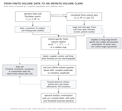
Finite-volume information reaches an infinite-volume claim only through a branch-specific map. Solid arrows show the controlled chain; dashed arrows show the long-range alternative and the stop rule. The image is schematic, not to scale, and the displayed determinant is structural: its channel, irrep, partial-wave, normalization, and sign conventions must be fixed locally.
The branch-status map adds a second distinction: elastic real-axis control does not automatically validate coupled-channel, current-insertion, or three-particle extensions. Each frontier branch carries its own hypotheses, benchmarks, and dated evidence boundary.
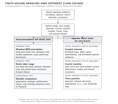
Finite-volume branches have different limits of interpretation. A fixed massless-field prescription and an exact power-law test are durable; mutable prescription comparisons may move to Research. Coupled-channel, current-insertion, and three-particle claims require separate dated status and validation. The map is schematic and not to scale.
Observable-level validation
Section titled “Observable-level validation”The finite-volume hypothesis and uncertainty table separates the real-axis quantization assumptions from the channel, sheet, and parametrization uncertainties that a pole continuation must also control.
Before accepting a pole extraction, verify that:
- every fitted energy obeys the elastic, short-range, frame, irrep, and partial-wave hypotheses;
- the amplitude form is exactly unitary on the real elastic axis and has no unreported physical-sheet singularity;
- correlated predicted energies reproduce all inputs and held-out levels;
- at least two analytically distinct unitary forms and a larger partial-wave basis fit acceptably;
- the sheet sign, crossed cuts, square-root branch, pole denominator, and residue normalization are recorded; and
- the pole distribution includes level covariance, common kinematics, parametrization alternatives, truncation, and continuation uncertainty.
What you can now do
Section titled “What you can now do”You can now (1) fit correlated elastic levels with two unitary amplitude forms and reproduce the levels by forward root solving, and (2) continue each fitted form to a named sheet and distinguish data-supported pole information from ansatz, threshold, sheet, and partial-wave assumptions.
Coupled-Channel Quantization and Inference adds threshold and sheet vectors. Physical resonance interpretation remains with Gauge Theories and the Standard Model, and dated comparative validation belongs to the Lattice and Hamiltonian Field Theory Research area.
Exercises
Section titled “Exercises”1. Unitary parametrization. Show that with real implies on the upper elastic bank.
Solution
The only imaginary term is because and are real there. Therefore , which is the inverse-amplitude form of elastic unitarity.
2. Pole versus fit parameter. Why is in the displayed matrix not generally ?
Solution
is a real-axis pole of one term in , while solves the full continued equation . Background terms, energy-dependent phase space, and nearby thresholds shift the complex solution. Only in an isolated narrow limit do the parameters approximately coincide.
References
Section titled “References”- Briceño, Raúl A., Jozef J. Dudek, and Ross D. Young. “Scattering Processes and Resonances from Lattice QCD.” Reviews of Modern Physics 90 (2018): 025001. DOI. Open PDF.
- Lüscher, Martin. “Two-Particle States on a Torus and Their Relation to the Scattering Matrix.” Nuclear Physics B 354 (1991): 531–578. DOI.