Blinding, Analysis Choices, and Independent Reproduction

Lattice analyses contain discretionary choices—fit windows, state counts, covariance conditioning, scale inputs, continuum ansätze, and exclusion rules. When those choices are influenced by the emerging target value, nominal statistical intervals no longer describe the complete selection process. Blinding, frozen decisions, structured alternatives, and independent analysis reduce this feedback without pretending that legitimate exploration can be eliminated.

Required background. Correlated fits and model selection identify influential choices, while equilibration and independent reproduction define independent histories and analysis implementations.

Map decisions before choosing a blind

Local analysis-control convention and regime. The estimand, diagnostics that must remain visible, discretionary decision nodes, blind transform, custodian, unblinding gate, and permitted post-unblinding actions are declared before production results are inspected. Exploration may inform a later frozen procedure but is not counted as confirmatory evidence. “Independent” always names which ensembles, derived data, code, libraries, priors, and analyst decisions are or are not shared.

List every choice from raw configurations to the final number, then mark its sensitivity and when it is made. Typical high-influence nodes are the thermalization cut, correlator window, covariance regularization, model set, ensemble exclusion, renormalization window, and continuum ansatz.

A blind should conceal the target while leaving diagnostics usable. Examples include:

• an unknown multiplicative factor for a positive amplitude;
• an additive offset for an energy or dimensionless result;
• hidden labels among analysis variants;
• withholding the final scale conversion;
• separating a selection dataset from a held-out target dataset.

The transform must preserve enough structure to debug code and inspect residuals. A multiplicative factor does not blind a dimensionless ratio in which it cancels; an additive offset can break a positivity or threshold diagnostic. Threat-model the actual analyst feedback path. Concrete blinding designs and failure modes in particle and nuclear physics are reviewed by Klein and Roodman 2005, pp. 141–163.

Frozen decisions and unblinding gates

Before revealing the target, record:

1. estimand and primary analysis;
2. ensemble inclusion and stationarity criteria;
3. autocorrelation and resampling rules;
4. fit windows, covariance treatment, and model alternatives;
5. scale, matching, and continuum procedures;
6. validation thresholds and conditions requiring revision;
7. the allowed actions after unblinding.

Unblind only after code tests, synthetic closure, intermediate invariants, and the independent review gate pass. If a post-unblinding change is scientifically necessary, preserve the original result, state the reason, classify the revision as exploratory or corrective, and obtain a new independent check. Quietly iterating until the preferred value appears defeats the control.

Structured alternatives

Predeclare a set of defensible analysis paths rather than selecting one by eye. Let $\widehat\theta_m$ denote the result from path $m$. The ensemble of paths exposes sensitivity, but it is not automatically a probability distribution. A combination rule—model weights, envelope, random-effects model, or worst-case bound—must match the scientific interpretation and be tested for coverage.

Alternative paths should vary one conceptual choice at a time where possible. Do not create dozens of nearly identical variants and count them as independent evidence. Track shared data, code, priors, and fit assumptions.

Independent reproduction

An independent analyst should receive the estimand, frozen inputs, and validation rules, not the preferred sequence of intermediate choices. Compare intermediate artifacts—averages, covariance eigenvalues, fit residuals, scale factors, and continuum inputs—before comparing only the final number.

Independence has degrees. Different wrappers around one fitting library catch fewer errors than different implementations; different implementations on the same ensemble do not test generation; independently regenerated ensembles with a shared analysis do not test that analysis. State the overlap.

The dependency graph shows blinding and independent analysis as cross-cutting tests, not a new statistical error added at the end.

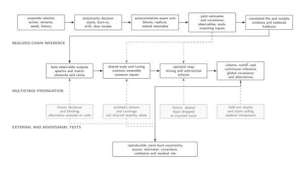
Frozen decisions and blinding control feedback into fits and model choices; independent implementations and held-out data test the resulting pipeline. These controls expose bias but are not uncertainty components to add mechanically. The diagram is schematic.

Exploration and confirmation

Exploration is valuable for discovering observables, windows, and models. Label it and separate it from confirmatory uncertainty, as emphasized by MacCoun and Perlmutter 2015, pp. 187–189. A practical sequence is:

1. explore on pilot or synthetic data;
2. freeze the primary and alternative analyses;
3. apply them blind to the production data;
4. unblind once gates pass;
5. validate on a held-out observable, ensemble, or independent implementation.

If no holdout is feasible, propagate the full adaptive selection through repeated synthetic experiments that resemble the decision process, and state the residual limitation.

Adversarial failure: the blind cancels from the target

Suppose a correlator is blinded by an unknown positive factor, $C_b(t)=\kappa C(t)$. The effective energy remains

$$aE_{\mathrm{eff},b}(t) =\log\frac{C_b(t)}{C_b(t+a)} =\log\frac{C(t)}{C(t+a)} =aE_{\mathrm{eff}}(t),$$

so the analyst can still see the target and tune the fit window toward it. The blind has changed a nuisance amplitude but not the estimand. Before production use, apply the proposed transform to a synthetic fixture and verify quantitatively that it conceals the target while preserving the residual, positivity, and threshold diagnostics needed for validation; otherwise the blinding gate must fail.

Observable-level validation checklist

• Enumerate every material discretionary choice from configurations to the quoted observable and rank its influence with frozen sensitivity tests.
• Verify on synthetic data that the blind changes the actual estimand, cannot be inferred from intermediate outputs, and preserves required diagnostics.
• Freeze the primary analysis, alternatives, validation thresholds, unblinding gate, and allowed corrective actions in a dated decision record.
• Repeat the complete adaptive selection procedure on synthetic or held-out data and measure bias plus interval coverage.
• Compare intermediate means, covariance eigenvalues, residuals, scales, and continuum inputs across independent implementations before comparing only final values.
• State the shared dependencies of every reproduction and preserve both pre- and post-unblinding results when a correction is necessary.

Common pitfalls

Blinding only the final plot label. If intermediate ratios or fit choices reveal the answer, analyst feedback remains possible.

Treating preregistration as proof of correctness. A frozen wrong method is still wrong. Closure and physical validation remain necessary.

Hiding post-unblinding changes. Preserve both versions and explain the scientific reason and new validation.

Learning outcomes

1. Given a lattice analysis dependency graph, identify every discretionary choice and design a blind or frozen-decision control whose effect on the target and diagnostics is verified on a synthetic fixture.
2. Given two nominally independent results, classify their shared ensembles, code, and decisions and quantify whether independent analysis changes or confirms the claimed uncertainty without concealing exploration.

Exercises

1. Why does multiplying all correlators by an unknown factor fail to blind an extracted energy?

Solution

Effective energies and exponential slopes depend on time ratios or logarithmic derivatives, so the common amplitude cancels. An energy offset or hidden scale may be needed instead.

2. Is agreement between two analysts using the same covariance file and fit library fully independent?

Solution

No. It tests some data handling and choice differences but shares covariance construction and fitting defects. Report the shared components and add an implementation or synthetic check if they matter.

References

• Klein, J. R., and Roodman, A. (2005). Blind analysis in nuclear and particle physics. Annual Review of Nuclear and Particle Science, 55, 141–163. DOI.
• MacCoun, R., and Perlmutter, S. (2015). Blind analysis: hide results to seek the truth. Nature, 526, 187–189. DOI.