Gauge Ensembles and Renormalized Observables

A stored gauge configuration is not yet a physical measurement. A renormalized observable is obtained only after connecting the path-integral measure, a finite-lattice operator, quantum-number projection, correlated estimation, scale setting, operator renormalization or subtraction, volume control, and continuum extrapolation. This page traces that chain without folding algorithmic, operator, and fit uncertainties into one opaque error bar.

Required background. The Wilson gauge action defines the measure, and Euclidean correlators define the spectral inference step.

Helpful background. Lines of constant physics and Markov-chain sampling provide the continuum and statistical controls.

From path integral to ensemble estimator

Local convention and regulator card. Fix the action, bare parameters, lattice geometry, boundary sector, stored-configuration spacing, and any reweighting factors before defining an estimator. For each observable, state its finite-lattice operator, symmetry and momentum projection, scale input, renormalization scheme and scale, subtraction basis, and the common resampling unit used to retain ensemble, scale, and matching covariance.

For an observable $O[U]$,

$$\langle O\rangle=\frac1Z\int[dU]\,O[U]e^{-S[U]}.$$

Given a stationary Markov chain $U_1,\ldots,U_N$, the sample mean

$$\overline O=\frac1N\sum_{i=1}^N O[U_i]$$

is consistent under ergodicity, but its variance is not $\operatorname{var}(O)/N$ for correlated samples. With integrated autocorrelation time $\tau_{\mathrm{int},O}$ in stored-configuration units,

$$\operatorname{var}(\overline O)\simeq \frac{2\tau_{\mathrm{int},O}}{N}\operatorname{var}(O).$$

The relevant autocorrelation time is observable dependent. Plaquette decorrelation does not establish adequate sampling of topological charge or a long-distance correlator.

Windowing and automatic-error procedures for correlated Markov data are derived in Wolff 2004, pp. 143–153; slow topological modes and their effect on lattice-QCD errors are analyzed in Schaefer, Sommer, and Virotta 2011, pp. 93–119.

If configurations carry reweighting factors $w_i$, use $\sum_iw_iO_i/\sum_iw_i$ and propagate numerator–denominator covariance. A small effective reweighting sample size is a loss of support, not a nuisance that bootstrap resampling can repair.

Operators, projection, and disconnected sectors

A correlator begins with a finite-lattice operator $O_\alpha$ whose symmetry channel, smearing, representation, and normalization are explicit. Momentum projection on a periodic spatial volume is

$$O_\alpha(\mathbf p,t)=a_s^3\sum_{\mathbf x} e^{-i\mathbf p\cdot\mathbf x}O_\alpha(\mathbf x,t).$$

For vacuum quantum numbers, the connected correlator requires the same-ensemble subtraction

$$C_{\alpha\beta}(t)= \left\langle O_\alpha(t)O_\beta(0)^*\right\rangle -\left\langle O_\alpha\right\rangle \left\langle O_\beta^*\right\rangle.$$

Performing each average on unrelated resamples destroys covariance. Disconnected quark contractions add stochastic and solver errors; an unbiased estimator requires either exact solves or a correction for approximate solves. Store these components separately from gauge-ensemble variation.

Attaching scale and renormalization

Suppose a bare lattice matrix element $M^{\mathrm{bare}}_j(a)$ mixes among operators. In scheme $\mathcal S$ at scale $\mu$,

$$M_i^{\mathcal S}(\mu,a)= \sum_j Z_{ij}^{\mathcal S}(\mu,a) \left[M_j^{\mathrm{bare}}(a)-\sum_k c_{jk}(a)M_k^{\mathrm{sub}}(a)\right].$$

The covariance of $M^{\mathrm{bare}}$, $Z$, subtraction coefficients, and the common scale must be propagated jointly. Multiplying central values by a separately sampled $Z$ and then adding percentage errors in quadrature is valid only if independence has been established.

Dimensionful results share the uncertainty of the scale-setting observable. If $Q=a^{-d}\widehat Q$, then infinitesimally

$$\frac{\delta Q}{Q}=\frac{\delta\widehat Q}{\widehat Q}-d\frac{\delta a}{a},$$

so all quantities from the same ensembles acquire common covariance through $a$.

One traceable analysis record

Stage	Object	Correlations retained	Required cross-check
Ensemble measure	Action, masses, volume, boundary sector	Shared configurations	Reversibility or independent kernel benchmark
Operator	Paths, smearing, irrep, source geometry	Same-noise and same-source correlations	Symmetry and gauge-transformation tests
Spectral inference	Correlation matrix and fit model	Time, channel, ensemble covariance	Fit-window and basis changes
Scale	Dimensionless reference quantity	Common ensemble and fit inputs	Alternative reference or ratio closure
Operator map	$Z_{ij}$ and subtractions	Shared gauge fields and matching data	Scheme/window/step-scaling variation
Limits	Volume and spacing sequence	Global correlated fit	Leave-one-spacing-out and volume comparison

Blinding a multiplicative factor or selected result can reduce analyst bias, but the rule and unblinding criterion must be fixed before viewing the target. Blinding does not compensate for a missing continuum or covariance model.

The branch structure below is part of the dependency analysis: all observables can share configurations and scale inputs while retaining different definition and validity uncertainties.

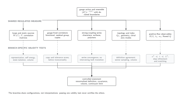
Shared ensembles create covariance, not equivalence. Each gauge-observable branch carries its own estimator and regime tests into the final renormalized, finite-volume, and continuum analysis. The diagram is schematic and not to scale.

Continuum target and uncertainty decomposition

Use dimensionless matched data $R_e$ from ensembles $e$ and a correlated model such as

$$R_e=R_\star+c_a(a_e\Lambda)^p+c_L e^{-mL_e} +c_m\delta m_e+\cdots.$$

Report identifiable uncertainty components: finite sampling and stochastic estimation; spectral or fit-model choice; scale and renormalization; finite volume; cutoff extrapolation; and external inputs. Some components are correlated and must not be counted twice. Model averaging or alternative fits should use a predeclared rule and expose which choices move the result.

The final label must match the attained stage: “bare at $a=0.08\,\mathrm{fm}$,” “renormalized at finite spacing,” or “continuum extrapolated in scheme $\mathcal S$ at $\mu$” are distinct claims.

Adversarial failure: shared scale fluctuations erased by separate fits

Let a dimension-$d$ result be $Q=a^{-d}\widehat Q$, with both $a$ and $\widehat Q$ determined on the same configurations. Construct a sample in which $\delta\log\widehat Q=d\,\delta\log a$ on every resample. Then

$$\delta\log Q=\delta\log\widehat Q-d\,\delta\log a=0,$$

so the scale-induced fluctuation cancels exactly. An analysis that fits $a$ and $\widehat Q$ separately and assumes independence instead assigns a nonzero variance equal to the sum of two terms. With the opposite correlation it can underestimate the variance. Agreement of central values therefore does not validate a pipeline that discards shared resampling information.

Observable-level validation checklist

• Recompute the operator on a gauge-transformed configuration and verify the expected invariant or covariant transformation law.
• Test symmetry, irrep, momentum, and vacuum-subtraction projections on configurations for which the answer is exactly known.
• Estimate autocorrelation times for the target correlator, topology when relevant, scale observable, and reweighting factor, then choose a common valid resampling block.
• Propagate $M^{\mathrm{bare}}$, subtraction terms, $Z_{ij}$, and the scale through the same correlated replicas or a verified joint covariance model.
• Repeat spectral, volume, renormalization-window, and cutoff analyses and require the final renormalized observable—not only an intermediate fit—to remain stable.

Common pitfalls

Using one autocorrelation time for every observable. Slow topology can coexist with a rapidly decorrelating plaquette. Diagnose the actual observable and relevant modes.

Renormalizing after an uncorrelated fit. Shared scale and $Z$ inputs couple ensembles and channels. Carry them as nuisance variables or propagate their full covariance.

Double-counting an uncertainty. If the scale enters both the abscissa and ordinate of a fit, adding a separate final scale percentage may count it twice.

Learning outcomes

1. Given configurations and a finite-lattice operator, construct a correlated estimator through projection, subtraction, scale setting, and operator mixing while retaining every shared covariance.
2. Given a reported result, classify it as bare, finite-spacing renormalized, or continuum extrapolated and design observable-level autocorrelation, volume, matching, and cutoff tests that could falsify that label.

Exercises

1. A chain has $N=2000$ stored measurements, variance $9$, and $\tau_{\mathrm{int}}=12$ configurations. Estimate the standard error of the mean.

Solution

$\sqrt{2\tau_{\mathrm{int}}\operatorname{var}(O)/N}=\sqrt{24\times9/2000}\simeq0.329$.

2. Two dimension-one observables share the same scale with relative uncertainty $s$. What scale-induced correlation do they have to first order?

Solution

Both receive the same fractional shift $-\delta a/a$, so their scale-induced covariance is $Q_1Q_2s^2$ and this component is perfectly positively correlated.

References

• Schaefer, S., Sommer, R., and Virotta, F. (2011). Critical slowing down and error analysis in lattice QCD simulations. Nuclear Physics B, 845, 93–119. DOI.
• Wolff, U. (2004). Monte Carlo errors with less errors. Computer Physics Communications, 156, 143–153. DOI.

Further reading

• Lüscher, M. (2010). Properties and uses of the Wilson flow in lattice QCD. Journal of High Energy Physics, 2010(08), 071. DOI.