

Hamiltonian Continuum Limits and Euclidean Cross-Validation
Hamiltonian and Euclidean regulators support a universality claim when they are tuned to the same renormalized target and yield compatible dimensionless observables after their distinct cutoffs are removed. Agreement at one finite lattice can diagnose conventions; it cannot establish a continuum limit. A useful cross-validation exposes shared inputs and decomposes discrepancies by spacing, volume, local Hilbert dimension, basis, temporal reconstruction, and operator matching.
Required background. Transfer matrices define finite-regulator Euclidean spectral comparisons; real-time observable extraction defines the Hamiltonian outputs; lines of constant physics define the continuum fit.
Helpful background. Complete lattice error budgets supply covariance and model-stability controls.
Match the target before comparing numbers
Section titled “Match the target before comparing numbers”Cross-formulation comparison card. Euclidean and Hamiltonian calculations share only the renormalized target and dimensionless continuum observable. Each retains its own spacing, volume, temporal, local-Hilbert, basis, sector, operator, and scheme data. Formulation-specific cutoff coefficients are fit separately, shared inputs carry covariance, and only a justified continuum intercept is common.
For each formulation, record the field normalization, spatial boundary condition, masses and couplings used as renormalization conditions, operator definition, scale, scheme, and order of limits. Equal-time periodic length and light-front longitudinal length , for example, are different finite regulators even if both eventually target the same invariant mass.
Choose dimensionless observables , such as mass ratios, normalized matrix elements, or a propagator at fixed physical . A joint model can be written
where labels the formulation and only the continuum intercept is shared. Forcing common cutoff coefficients between unrelated regulators creates artificial agreement.
The need for formulation-specific cutoff expansions and controlled continuum extrapolation follows the effective-action analysis of Symanzik 1983, pp. 187–204.
Exact free-scalar closure test
Section titled “Exact free-scalar closure test”For the one-dimensional spatial scalar lattice,
The Hamiltonian ground-state covariance is
The zero-frequency Euclidean propagator in the same field convention is
This equality closes the normalization loop at finite spatial regulator. At in the continuum, , while the one-particle gap satisfies . A projected local oscillator basis must first reproduce the exact finite-chain covariance and gap as increases; only then should its residual spacing dependence be compared with Euclidean data.
The volume’s formulation map shows the larger evidence chain.
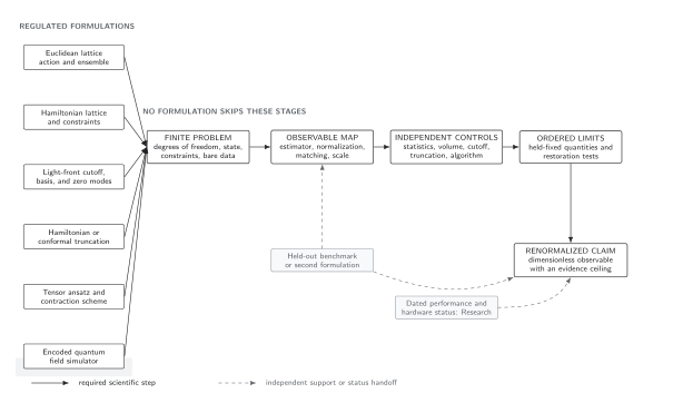
Cross-formulation agreement is the final gate after each regulator has passed its own tuning and limit tests. A common target and observable are required before numerical values are compared. The diagram is schematic.
The Hamiltonian-specific map resolves the physical-sector and observable branches within that larger chain.
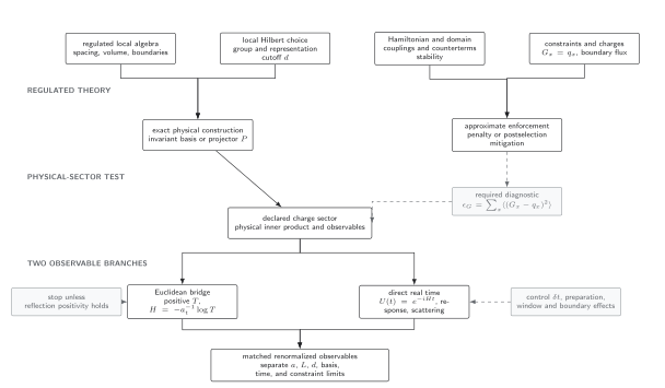
Euclidean transfer data and direct real-time data become common evidence only after physical-sector, operator, scale, and renormalization matching. Each regulator axis remains visible in the final comparison. The diagram is schematic.
Matched comparison table
Section titled “Matched comparison table”| Item | Euclidean route | Hamiltonian route | Shared comparison | Failure diagnosis |
|---|---|---|---|---|
| Target | action and tuned bare parameters | and counterterms | same renormalized conditions | different theory or convention |
| Spectrum | exponential correlator decay | energy differences | dimensionless gaps and dispersion | positivity, excited state, , or basis effect |
| Matrix element | two- and three-point functions | state overlap or response | same renormalized operator | normalization or mixing mismatch |
| Propagator | Matsubara or Euclidean momentum | spectral sum or equal-time covariance | fixed physical | frequency convention or finite window |
| Constraints | Ward identities and gauge invariance | projector weight and | same charge sector | leakage or boundary mismatch |
| Limits | common intercept only | hidden or noncommuting cutoff | ||
| Covariance | shared ensembles and scale | shared tuning and benchmarks | joint nuisance parameters | correlated error counted twice |
Diagnosing a discrepancy
Section titled “Diagnosing a discrepancy”Proceed from exact to asymptotic checks:
- verify units, Fourier conventions, field normalization, and boundary sectors;
- compare exact free or small-system results at the same finite regulator;
- close local-dimension, basis, time-step, and constraint errors within the Hamiltonian route;
- close temporal, statistical, and spectral-fit errors within the Euclidean route;
- compare volume sequences at matched physical ;
- fit spatial cutoff effects with independent formulation-specific terms;
- test a held-out observable and an alternative discretization.
If the discrepancy persists only in the continuum intercept and survives these tests, it may indicate a mistuned relevant coupling, unmatched operator, noncommuting limit, or genuinely different universality class. It should not be absorbed into an inflated undifferentiated systematic error.
Adversarial failure case
Section titled “Adversarial failure case”Tune the lowest gap independently in both formulations, include that same gap as the dominant datum in a joint fit, and impose a common coefficient. The fit can report a precise shared intercept even if a held-out matrix element has opposite cutoff trends, because the tuned datum and restrictive prior manufacture agreement. Remove tuning observables from the validation set, allow formulation-specific cutoff terms, propagate their shared scale covariance, and require a withheld observable or regulator point to close.
Observable-level validation
Section titled “Observable-level validation”The equal-time regulator comparison table summarizes which quantities remain fixed and which tests accompany each regulator limit before a cross-formulation comparison.
- Match field, state, charge-sector, operator, scale, scheme, and boundary conventions before comparing any numerical value.
- Reproduce a free or exactly diagonalizable quantity at the same finite regulator on both routes.
- Close local-dimension, basis, time-step, constraint, temporal-fit, and finite-volume errors within their respective formulations.
- Fit formulation-specific cutoff dependence with shared nuisance parameters and covariance only where the inputs are genuinely common.
- Predict a held-out dimensionless observable and at least one withheld regulator point before accepting a common continuum intercept.
Common pitfalls
Section titled “Common pitfalls”Identifying unequal finite boxes. Different quantization surfaces and compact directions have different spectra. Compare common continuum observables, not nominal box lengths.
Using the exact continuum value as a fit prior and then claiming validation. Hold out at least one quantity or regulator sequence not used in tuning.
Treating formulation results as statistically independent. Shared masses, scale inputs, perturbative coefficients, or exact benchmarks create covariance that belongs in the combined model.
Learning outcomes
Section titled “Learning outcomes”- Construct a matched Euclidean–Hamiltonian comparison table that fixes the renormalized target, dimensionless observables, sector, scheme, scales, covariance, and independent limit order.
- Given a persistent discrepancy, use finite-regulator closure tests and a held-out observable to classify it as spacing, volume, local-Hilbert, basis, time, constraint, operator-matching, or target-theory error.
Exercises
Section titled “Exercises”- Verify for the continuum free scalar.
Solution
, so at it equals .
- Two formulations agree at one spacing after tuning the gap. Name a useful held-out check.
Solution
A propagator at fixed physical momentum, a matrix element, or a second dispersion point tests field/operator normalization and cutoff structure not fixed by the gap. It should be repeated across spacings and volumes.
References
Section titled “References”- Symanzik, K. (1983). Continuum limit and improved action in lattice theories. I. Principles and theory. Nuclear Physics B, 226, 187–204. DOI.