Complex Langevin and Stochastic Correctness

Complex Langevin replaces integration against a complex weight on real fields by a real, positive probability distribution over complexified fields. Convergence of the stochastic process is not the correctness criterion. Correctness requires the formal integration-by-parts argument to survive noncompact excursions and drift singularities, the process to sample every relevant stationary component, and holomorphic observables to agree with exact or sign-free references in a demonstrated parameter range.

Required background. Anatomy and severity of a sign problem supplies the distinction between variance and bias. Brownian motion, stochastic calculus, Langevin, and Fokker–Planck equations supplies Itô evolution.

Helpful background. Algorithm validation and ensemble provenance supplies stationarity, autocorrelation, and reproducibility tests.

Complexified stochastic evolution

Convention and regulator card. Begin with a finite-dimensional regulated integral $Z=\int_{\mathbb R^n}dx\,e^{-S(x)}$. Complexify $z=x+iy$ and assume the action and measured observables have holomorphic continuations except at explicitly tracked determinant zeros or logarithmic branch points. Langevin time $t_L$ is algorithmic, not Euclidean or physical time. The equations below use real noise with $\langle dW_i,dW_j\rangle=\delta_{ij}dt_L$.

The stochastic differential equation is

$$dz_i=K_i(z)dt_L+\sqrt2\,dW_i, \qquad K_i(z)=-\partial_{z_i}S(z).$$

For a holomorphic observable $O(z)$, Itô’s formula gives

$$\frac{d}{dt_L}\langle O\rangle_P =\langle LO\rangle_P, \qquad L=\sum_i(\partial_{z_i}+K_i)\partial_{z_i},$$

where $P(x,y;t_L)ge0$ is the probability density generated in complexified space. A stationary trajectory should satisfy the Schwinger–Dyson-like identities

$$\langle LO\rangle_P=0$$

for a sufficiently rich set of observables. These identities are necessary but not sufficient: a wrong stationary solution can satisfy a limited test set.

Where the formal proof can fail

The justification compares evolution under $P(x,y;t_L)$ with evolution of a complex density $ρ(x;t_L)$ on the original contour. Repeated integration by parts moves the Fokker–Planck operator from the density onto $O$. Equality requires every surface term to vanish at $|y|\to\infty$, at large real fields, and around poles of $K$. If $P$ decays too slowly or the process frequently approaches a drift pole, the equality can fail even though time series are stationary. Boundary terms near infinity and poles have been exhibited directly in solvable models Scherzer et al. 2019.

A practical necessary diagnostic is the magnitude of the drift,

$$u(z)=\left(\frac1n\sum_i|K_i(z)|^2\right)^{1/2}.$$

Power-law tails in the empirical distribution of $u$ are incompatible with the decay used in the formal argument; an exponential-or-faster drift tail is a sharper criterion under the assumptions analyzed by Nagata, Nishimura, and Shimasaki 2016. Passing a fitted tail test remains one piece of evidence, not a universal theorem for an interacting lattice simulation.

Fermion determinants make the drift meromorphic:

$$S_{\rm eff}=S_g-N_f\log\det D, \qquad K\supset N_f\operatorname{Tr}(D^{-1}\partial D).$$

Zeros of $\det D$ are drift poles. Choosing a branch for $\log\det D$ does not remove the pole in its derivative. One must monitor the smallest singular values or determinant-zero distance together with $u$.

Gauge cooling and stabilization

For gauge fields, complexification enlarges $SU(N)$ to $SL(N,\mathbb C)$. Gauge cooling applies complexified gauge transformations to reduce a nonunitarity norm while leaving gauge-invariant holomorphic observables unchanged. It can suppress excursions and make the boundary decay plausible; under stated conditions it can be incorporated into the justification Nagata, Nishimura, and Shimasaki 2016, gauge-cooling analysis.

Cooling is not a projection back to the unitary manifold, does not remove determinant zeros, and does not prove ergodicity. “Dynamic stabilization” or drift modification changes the stochastic equation; unless the added term is shown to vanish in a controlled limit with observable stability, it introduces a method bias that must be extrapolated.

Exact benchmark with a nearby pole

For the one-angle fixture, choose the holomorphic action

$$S(z)=-\beta_0\cos z -\log(1+he^{\mu+iz}) -\log(1+he^{-\mu-iz}).$$

The drift is

$$K(z)=-\beta_0\sin z +\frac{ihe^{\mu+iz}}{1+he^{\mu+iz}} -\frac{ihe^{-\mu-iz}}{1+he^{-\mu-iz}}.$$

It has poles where either bracket vanishes. One family is

$$z=(2k+1)\pi-i(\log h^{-1}-\mu).$$

With $h=0.2$, a pole approaches the original real contour as $μ\to\log5\simeq1.609$. Therefore the prescribed points $μ=0.5,1,1.5$ intentionally move from easy to hostile drift geometry.

A benchmark run measures the density $n=\partial_\mu\log Z_1$ and Fourier observables $e^{ikz}$, comparing with exact Bessel formulas. Record step-size extrapolation, drift histogram, imaginary excursion, pole distance, $⟨LO\rangle$ for several $k$, and dependence on initial conditions. A trajectory at $μ=1.5$ can look stationary while sampling on one side of a pole and giving the wrong density; this is the required “converged but incorrect” negative control.

Correctness protocol

1. Discretization: run several adaptive maximum steps and extrapolate the Langevin step to zero.
2. Stationarity and mixing: compare dispersed initial conditions, long blocks, symmetry-related sectors, and autocorrelation times.
3. Holomorphic identities: test $\langle LO\rangle=0$ for a growing basis of bounded-degree observables, not only the action.
4. Boundary control: inspect field, unitarity-norm, drift, and determinant-zero tails; estimate explicit boundary terms where feasible.
5. Reference values: reproduce exact small systems, imaginary-μ or other sign-free regimes, and a known-failure region.
6. Scaling: repeat diagnostics with volume, lattice spacing, masses, and $μ$; a safe window can shrink.

No single item licenses correctness alone. In particular, agreement with one low-order observable can coexist with wrong higher moments, and small $⟨LO\rangle$ can reflect an incomplete observable basis.

Adversarial failure cases

Stationary wrong limit. Means and histograms stop drifting, but a nonzero boundary term invalidates the formal proof. Compare with exact data and measure boundary observables rather than extending run length alone.

Adaptive steps hide singular drift. Reducing steps prevents numerical blow-up near a pole but does not make visits harmless. Report the drift tail and pole-distance distribution before and after adaptation.

Cooling norm becomes the target. Aggressive cooling produces a small unitarity norm while a gauge-invariant observable is wrong. Cooling is a stability device; exact references and correctness identities remain mandatory.

One initial condition misses a stationary component. Run hot, cold, and symmetry-related starts and test transitions between modes. Agreement of their action densities is weaker than agreement of phase-sensitive observables.

The correctness map below shows why stationary-looking complex-Langevin data do not close the proof. Follow its branch through holomorphy, drift tails, boundary terms, pole encounters, and exact fixtures before comparing it with methods governed by different conditions.

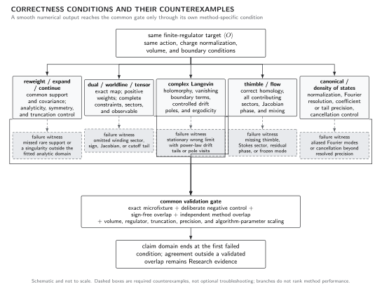
Each reformulation has a different correctness condition and a characteristic counterexample. Apparent numerical convergence is insufficient when overlap is absent, a dual sector or Jacobian is missing, complex-Langevin boundary terms survive, a contributing thimble is omitted, or canonical and density-of-states cancellations exceed resolved precision. The map is schematic and does not rank current algorithms.

Observable-level validation checklist

• State the complexification, drift, noise convention, integrator, adaptive rule, cooling or stabilization term, and step-size limit.
• Publish drift and excursion tails, determinant singular-value diagnostics, and several $\langle LO\rangle$ identities.
• Reproduce exact and sign-free observables plus a parameter point where the method is expected to fail.
• Test initial-condition dependence, multimodality, autocorrelation, volume scaling, and regulator scaling.
• Mark results outside the demonstrated diagnostic window as uncontrolled Research evidence, even if trajectories are smooth.

Exercises

1. Langevin identity

For one variable and $O(z)=z^2$, derive $LO$.

Solution

Since $\partial_zO=2z$ and $\partial_z^2O=2$,

$$LO=(\partial_z+K)\partial_z z^2=2+2zK(z).$$

A stationary correct process must therefore satisfy $\langle1+zK(z)\rangle=0$, provided the relevant moments and boundary manipulations exist.

2. Pole location

Solve $1+he^{\mu+iz}=0$ and determine its distance from the real contour for $h=0.2$ and $μ=1.5$.

Solution

Write $he^{\mu+iz}=e^{\log h+\mu+i\operatorname{Re}z-\operatorname{Im}z}=-1$. Thus $\operatorname{Re}z=(2k+1)\pi$ and $\operatorname{Im}z=\mu-\log h^{-1}$. The distance is $\log5-1.5\simeq0.109$, so pole encounters are a serious diagnostic at that point.

Learning outcomes

After working this page, you should be able to:

• Derive the complex Langevin operator and test a basis of stationary identities while locating every drift singularity of a regulated model.
• Reproduce one correct and one converged-but-incorrect benchmark and decide the validated parameter window from tail, pole, mixing, and exact-comparison evidence.

Handoff

Lefschetz thimbles and holomorphic flow use deterministic contour geometry instead of stochastic complexification. Cross-method validation sets the claim ceiling when either method is compared with sign-free or exact data.

References

• Nagata, Keitaro, Jun Nishimura, and Shinji Shimasaki. “Argument for Justification of the Complex Langevin Method and the Condition for Correct Convergence.” Physical Review D 94 (2016): 114515. doi:10.1103/PhysRevD.94.114515.
• Nagata, Keitaro, Jun Nishimura, and Shinji Shimasaki. “Justification of the Complex Langevin Method with the Gauge Cooling Procedure.” Progress of Theoretical and Experimental Physics 2016 (2016): 013B01. doi:10.1093/ptep/ptv173.
• Scherzer, Manuel, Erhard Seiler, Dénes Sexty, and Ion-Olimpiu Stamatescu. “Complex Langevin and Boundary Terms.” Physical Review D 99 (2019): 014512. doi:10.1103/PhysRevD.99.014512.