

Entanglement Structure and Tensor-Network Ansätze
A tensor-network ansatz is a finite-regulator representation of a state or partition function whose graph fixes which indices may carry correlations and whose bond dimensions bound the retained Schmidt ranks. Locality and entanglement guide the graph, but they do not prove efficient approximation; bond truncation, local-field truncation, finite volume, lattice spacing, and optimization remain distinct approximations.
Required background. Direct sums, tensor products, and index structure supplies tensor-factor and contraction notation.
Helpful background. Variational principles and field-theory ansätze supplies the Rayleigh–Ritz logic used for state optimization. Fock space, vacuum, and particle number supplies the occupation-space interpretation of a local field cutoff.
Tensor graphs as regulated factorizations
Section titled “Tensor graphs as regulated factorizations”Let a spatial lattice have local basis , . A general coefficient tensor has entries,
An open-boundary matrix product state (MPS) factorizes it as
with . A projected entangled-pair state (PEPS) uses one virtual index per incident spatial bond; MERA adds a scale direction through isometries and disentanglers. A Euclidean tensor network has a different object at its center: all indices are contracted to produce or an insertion numerator, rather than leaving physical indices for a wavefunction. A practical comparison of MPS and PEPS representations, canonical forms, and contraction strategies is developed by Orús 2014.
Regulator and convention box. The Hamiltonian and local basis are fixed before choosing a network. Record the lattice spacing , spatial size , boundary conditions, local dimension , graph , every bond dimension , symmetry sectors, tensor normalization or canonical gauge, and optimizer stopping rule. A change of virtual gauge is not a physical cutoff change. A change of is not a bond-dimension change.
For any cut crossed by virtual bonds, the Schmidt rank obeys
The inequality explains why MPS match one-dimensional area-law states and why PEPS have an area-compatible virtual boundary. It is only an expressivity ceiling. It neither guarantees that optimization finds the needed tensors nor bounds the error of a local observable. The distinction is emphasized in the structural treatment of MPS and PEPS by Cirac et al. 2021, §§ II–III.
Schmidt decomposition and the bond regulator
Section titled “Schmidt decomposition and the bond regulator”Across one cut, write
Keeping the first terms gives the best rank- approximation in the Hilbert norm for this one bipartition,
Successive Schmidt decompositions yield an exact MPS when no rank is truncated. Once truncations are made at several cuts, the local discarded weights are valuable diagnostics but are not automatically a rigorous error bar for a later nonlinear optimization, a PEPS contraction, or a continuum-extrapolated observable. Schollwöck 2011, §§ 4.1–4.5 develops the canonical-form and truncation construction.
MPS tensors have a representation gauge:
which leaves every coefficient unchanged for invertible . Canonical gauges turn this redundancy into useful orthonormality conditions. A large gradient along a gauge orbit is therefore not a physical residual; conversely, a small coordinate gradient before gauge fixing need not imply a well-optimized state.
The geometry–object distinction and the independent limits to inspect are summarized below. Follow the state branch for MPS, PEPS, or real-time work and the partition-function branch for Euclidean tensor renormalization.
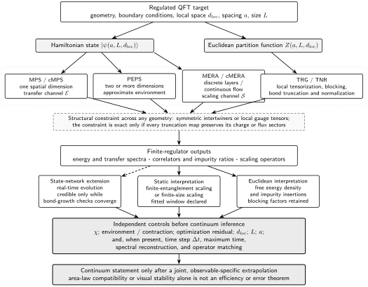
Tensor geometry is selected from the regulated object and dimension, not from a universal efficiency claim. The diagram is schematic and not to scale: all routes retain separate bond, contraction, optimization, local-space, volume, spacing, and—where present—time controls before a continuum statement.
Exactly checkable two-site scalar fixture
Section titled “Exactly checkable two-site scalar fixture”Truncate each of two scalar oscillators to and consider the normalized even-parity state
Its coefficient matrix is diagonal, so the Schmidt coefficients are exactly and . A bond- truncation keeps , has discarded weight , fidelity , and entropy
At the regulated vacuum is a product state and is exact. For any , loses the connected number correlation:
even though the retained state has a perfectly well-defined variational energy. This fixture isolates bond error at fixed ; raising the oscillator cutoff is a separate test.
Method contract from target to claim
Section titled “Method contract from target to claim”- Specify the regulated Hamiltonian state or Euclidean partition function and the target observable.
- Choose a graph from dimension, locality, expected entanglement, and the operation to be performed—not from an area-law slogan alone.
- Declare physical indices, virtual indices, orientation conventions, symmetry sectors, , and every .
- Fix or account for virtual gauge freedom before interpreting norms, gradients, or environments.
- Optimize or contract with a reproducible residual and multiple initializations where local minima are possible.
- Vary the bond regulator independently of , , , and contraction controls.
- Validate at a product point, free theory, exact small lattice, or another independently controlled formulation.
The chapter-wide tensor-network regulator and error record lists the declarations required before a result is promoted beyond its finite controls.
Adversarial failure: area law, wrong state
Section titled “Adversarial failure: area law, wrong state”A variational family may obey the same area-law upper bound as the target yet omit the target’s symmetry sector or topological virtual structure. Energy optimization can then settle into a low-energy state with the wrong charge, boundary flux, or long-distance correlator. The failure is exposed by enlarging the virtual sector content, changing the initialization, and measuring a held-out symmetry or flux observable—not by increasing within the same defective sector list.
Observable-level validation checklist
Section titled “Observable-level validation checklist”- Verify state norm or partition-function normalization in the chosen gauge.
- Compare an exact small-system Schmidt spectrum or contraction.
- Scan at fixed , , and ; then scan those physical regulators separately.
- Check charge, parity, Gauss law, or other structural constraints locally and globally.
- Report energy residuals and at least one held-out correlator; do not use the fitted energy as its own test.
- For approximate contraction, change the environment dimension and contraction family.
- State the strongest supported claim: exact finite-network identity, variational energy statement, empirical convergence, or continuum extrapolation.
What you should be able to do
Section titled “What you should be able to do”After this page, you should be able to:
- factor a regulated many-body coefficient tensor into a graph and label its physical, virtual, symmetry, and cutoff indices; and
- diagnose whether a discrepancy comes from virtual gauge, bond truncation, local Hilbert truncation, finite volume, lattice spacing, contraction, or optimization.
Exercises
Section titled “Exercises”1. Minimal bond dimension. For , find the Schmidt ranks across the cuts and , and hence the smallest open-MPS bond dimensions.
Solution
Across , the right states and are orthogonal, so the rank is two. Across , rewrite the state as ; the rank is also two. Thus is minimal.
2. Gauge invariance. Insert between neighboring MPS tensors and prove that the physical coefficient tensor is unchanged. Why can a condition number of still matter numerically?
Solution
The transformed product contains , so every coefficient is identical. In finite precision, an ill-conditioned amplifies rounding and makes local norms and gradients poorly scaled. Canonicalization changes numerical conditioning without changing the state.
References
Section titled “References”- Cirac, J. Ignacio, David Pérez-García, Norbert Schuch, and Frank Verstraete. “Matrix Product States and Projected Entangled Pair States: Concepts, Symmetries, Theorems.” Reviews of Modern Physics 93 (2021): 045003. DOI.
- Orús, Román. “A Practical Introduction to Tensor Networks: Matrix Product States and Projected Entangled Pair States.” Annals of Physics 349 (2014): 117–158. DOI.
- Schollwöck, Ulrich. “The Density-Matrix Renormalization Group in the Age of Matrix Product States.” Annals of Physics 326 (2011): 96–192. DOI.