Light-Front Regulators, Counterterms, and Symmetry Restoration

A truncated light-front Hamiltonian is controlled only when every regulator is declared, the operators it induces are included to a stated accuracy, their coefficients are fixed by independent renormalization conditions, and symmetries broken by the regulator are tested on held-out observables. Bare parameters generally flow with longitudinal, transverse, basis, and Fock- sector cutoffs. Sector-dependent parameters can organize a useful approximation, but they are not universal couplings and do not by themselves establish a regulator-independent theory.

Required background. DLCQ and Basis Light-Front Quantization supplies the independent finite-basis cutoffs. Light-Front Constraints, Zero Modes, and Vacuum Structure supplies the constrained operators that must survive renormalization. Symmetry Constraints and the Space of Counterterms supplies operator-basis construction from locality, power counting, and residual symmetries.

Helpful background. Regulator Removal and Renormalized Predictions supplies the distinction between fitting at finite regulator and demonstrating a regulator-independent prediction.

A regulated Hamiltonian is a family, not one matrix

Convention and regulator card. Coordinates use $x^\pm=(x^0\pm x^3)/\sqrt2$ and $M^2=2P^+P^- -\mathbf P_\perp^2$. Write $\boldsymbol\Lambda=(L_-,K,\delta,\Lambda_\perp,N_{\max},b,N_F,\ldots)$ for longitudinal volume and resolution, a possible small-$x$ cutoff, transverse or basis cutoffs, basis scale, and retained Fock sectors. Gauge fixing, pole prescriptions, regulator fields, zero modes, and boundary conditions are separate entries even when they do not fit in $\boldsymbol\Lambda$. Coefficients are compared only after matching the same scheme, scale, states, and observables.

The object to be renormalized is a family

$$P^-_{\boldsymbol\Lambda} =P^-_{0,\boldsymbol\Lambda} +\sum_a c_a(\boldsymbol\Lambda)\, \mathcal O_{a,\boldsymbol\Lambda}.$$

The operator set is determined before fitting. Start from the target theory, retain every operator allowed by the residual exact symmetries and the declared accuracy, and include structures generated by constraints or eliminated sectors. A light-front regulator can preserve longitudinal boosts while breaking rotations, or preserve a kinematical charge while violating a Ward identity. Consequently, a covariant counterterm list copied from an unregulated Lagrangian need not be complete for the finite Hamiltonian.

The following table is the light-front part of the chapter-spanning regulator comparison. The equal-time Hamiltonian part belongs to Chapter 9.

Light-front regulator, constraint, counterterm, limit, and validation requirements.

Regulator choice	Finite problem	Constraint or symmetry at risk	Induced operator obligation	Removal or convergence test	Held-out observable
$L_-$ and boundary condition	Compact longitudinal direction	Boundary charge, boost covariance, finite-volume physics	Boundary and zero-mode terms consistent with the chosen condition	Vary $L_-$ at fixed resolutions and renormalized inputs	Mass or current compared with an infinite-volume or independent-box result
Harmonic resolution $K$	Rational fractions $x_i=n_i/K$	Endpoint resolution and continuum longitudinal integrals	Consistent quadrature, self-energy, and vertex terms at each $K$	Fixed-$L_-$ $K$ sequence, separate from the volume sequence	Wavefunction moment or excited mass not used in tuning
Small-$x$ cutoff $x_i\ge\delta$	Endpoint singularities excluded	Boost, gauge, and zero-mode cancellations	Endpoint, instantaneous, and possibly nonlocal-in-$x^-$ counterterms	$\delta\to0$ with Ward and endpoint residuals monitored	Current component or scattering quantity sensitive to the endpoint
$\Lambda_\perp$ or $(N_{\max},b)$	Finite transverse momentum or oscillator space	Dynamical rotations, transverse boosts, locality	Anisotropic kinetic, vertex, and composite-current operators allowed by residual symmetry	Several cutoffs and $b$ values; compare a second transverse basis	Rotation multiplet splitting or frame-independent form factor
Fock-sector set $N_F$	Finite particle-content graph	Crossing, covariance, cancellations among time orderings	Induced self-energies, vertices, interactions, and currents from omitted sectors	Nested sector sets with one stated matching protocol	Scattering or current datum not used to fit sector parameters
Zero-mode prescription	Kernel of $\partial_-$ solved, constrained, or omitted	Vacuum branches, Gauss law, topology, spontaneous symmetry realization	Exact integrated constraint or its explicitly matched effective operator	Compare admissible prescriptions and the relevant limit order	Order parameter, Ward identity, or spectrum sensitive to the sector
Gauge and UV regulator fields	Gauge-fixed finite Hamiltonian, sometimes in an enlarged metric space	Ward identities, residual gauge invariance, unitarity	Gauge-restoring counterterms and regulator-field interactions	Regulator masses removed with negative-metric components decoupled	Charge, polarization independence, or physical scattering amplitude

The table is a structured equivalent of the figure below: each row starts from one regulator axis, names the lost information, and ends in a falsifiable observable rather than in a fitted coefficient.

Each regulator axis creates a distinct obligation

Inspect the four central arrows in the figure. Longitudinal, transverse, Fock-space, and gauge/UV regulators feed different constraint and symmetry problems before they can be combined in one counterterm Hamiltonian. The dashed return arrow means a failed held-out test forces the operator basis or matching conditions to be revised.

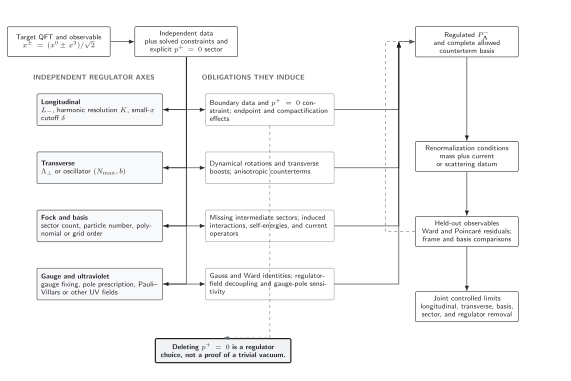
Each light-front regulator axis induces a different missing-information and counterterm problem. Renormalization conditions fix inputs, while held-out observables, Ward and Poincaré residuals, frame and basis comparisons, and simultaneous control of all limits test the result. The diagram is an original schematic and is not to scale; deleting the $p^+=0$ sector is explicitly shown as a regulator choice rather than a vacuum theorem.

The solid paths are necessary obligations, not a promise that a finite set of counterterms always suffices nonperturbatively. The allowed operator space and its power counting depend on the target theory and regulator. A calculation that cannot bound omitted operators must lower its accuracy claim.

Eliminated sectors generate interactions

Let $P$ project onto the retained Fock/basis space and $Q=1-P$. For an exact eigenstate $H|\Psi\rangle=E|\Psi\rangle$, the two projected equations give

$$Q|\Psi\rangle =\frac{1}{E-QHQ}\,QHP\,P|\Psi\rangle$$

whenever the resolvent exists with the required boundary prescription. Substitution yields the exact energy-dependent operator on the retained space,

$$H_{\mathrm{eff}}(E) =PHP +PHQ\frac{1}{E-QHQ}QHP.$$

Setting $Q|\Psi\rangle=0$ drops the second term. That term contains the self-energies, exchange interactions, many-body operators, and current corrections generated by omitted states. A practical counterterm expansion approximates it over a stated energy and observable domain; convergence of one eigenvalue does not show that the approximation works for another operator.

This projection identity also explains sector dependence. A self-energy in the highest retained sector lacks intermediate states available to a lower sector, so one bare mass can fail to cancel both. Allowing a mass or coupling to depend on the active Fock sector can compensate within the truncation. However, those sector-labeled coefficients should approach a common renormalized description, or their residual spread must enter the error. The formalism and its consistency conditions are developed in Karmanov, Mathiot, and Smirnov 2008, §§ II–III, pp. 085028-2–085028-7.

A scalar matching contract uses two inputs and a prediction

Consider a regulated $1+1$-dimensional $\phi^4$ Hamiltonian in a declared set of even and odd particle sectors. At a fixed approximation order, write

$$P^-_{\boldsymbol\Lambda} =P^-_0 +\frac{\delta m^2_{\boldsymbol\Lambda}}{2} \int\!\mathrm dx^-:\!\phi^2\!: +\frac{\lambda_{\boldsymbol\Lambda}}{4!} \int\!\mathrm dx^-:\!\phi^4\!: +\sum_r c_{r,\boldsymbol\Lambda}\mathcal O_r.$$

Here the $\mathcal O_r$ are all additional operators allowed by the residual symmetries and retained by the stated power counting: zero-mode- induced, derivative, sector-projector, and effective many-body terms are not silently absorbed into the two displayed coefficients. Normal ordering is part of the scheme, not a claim that every self-energy has vanished.

Choose two independent renormalization conditions, for example

$$M_1(\boldsymbol\Lambda)=m_R, \qquad \mathcal T_{2\to2}(s_0;\boldsymbol\Lambda)=\lambda_R$$

with the state normalization, kinematics, and definition of $\mathcal T$ fixed. Solve these conditions for two coefficient combinations. If more coefficients remain, supply more independent conditions or power- counting information; an underdetermined fit is not renormalization.

Then predict, without refitting, an excited mass, a second scattering energy, or a matched current matrix element. Repeat the complete procedure at a Cartesian set of $K$, $L_-$, transverse/basis, and sector cutoffs. Parameter stability is useful diagnostic information, but only held-out observable stability tests predictive control. Hamiltonian light-front counterterm construction and coupling coherence are discussed in Allen and Perry 1998, §§ II–VI, pp. 125017-2–125017-14 and surveyed in Hiller 2016, §§ 3.5–3.6, preprint pp. 29–38, PDF.

Symmetry restoration is measured, not asserted

An exact continuum representation satisfies

$$[G_A,G_B]=if_{AB}{}^C G_C$$

for the Poincaré generators. At finite cutoff, project the residual onto a low-energy test space $P_{\mathrm{test}}$ and report a dimensionless norm such as

$$r_{AB} =\frac{\left\|P_{\mathrm{test}} \left([G_A,G_B]-if_{AB}{}^CG_C\right) P_{\mathrm{test}}\right\|} {\left\|P_{\mathrm{test}}[G_A,G_B]P_{\mathrm{test}}\right\| +\left\|P_{\mathrm{test}}f_{AB}{}^CG_CP_{\mathrm{test}}\right\|+\epsilon}.$$

The small positive $\epsilon$ is declared and prevents an ill-defined $0/0$; it must not mask a small physical scale. Complementary tests include frame independence of $M^2$, degeneracy of states related by rotations, dispersion relations, and the angular condition for spinful currents.

For a conserved current, use

$$J_R^\mu =Z_JJ_{\mathrm{basis}}^\mu +\sum_a d_a(\boldsymbol\Lambda)\mathcal O_a^\mu,$$

and test both charge normalization and $q_\mu\langle f|J_R^\mu|i\rangle=0$. Matching only $J^+$ at $q^+=0$ can be efficient, but it does not establish equality of $J^+$, $J^-$, and transverse extractions when the truncation has broken covariance. The explicitly covariant light-front analysis shows how front orientation and the angular condition diagnose rotational dependence Carbonell et al. 1998, §§ 2.1–3.5, arXiv PDF pp. 8–55.

Adversarial failure: fitting away a broken symmetry

Suppose $\delta m^2_{\boldsymbol\Lambda}$ is fitted so the ground-state mass is exact at every $N_{\max}$. A rotation multiplet remains split and two current components give different form factors. Calling the mass plateau “symmetry restoration” confuses one renormalization input with two failed predictions.

The repair is to enlarge the allowed Hamiltonian and current operator bases, fix their coefficients with independent conditions, and reserve the multiplet splitting and component comparison as tests. If available counterterms cannot reduce both residuals with stable cutoff flow, the truncation has not reached the claimed accuracy.

Observable-level validation

• Completeness: document the residual symmetries, power counting, and every allowed Hamiltonian and current operator through the claimed order.
• Identifiability: use at least as many independent renormalization conditions as fitted coefficient combinations and report conditioning.
• No circularity: keep masses, scattering points, current components, or frames not used in fitting as held-out tests.
• Cutoff flow: vary longitudinal, transverse, basis-scale, Fock-sector, zero-mode, gauge, and regulator-field axes independently.
• Symmetry: report Poincaré commutator residuals, rotation multiplet splittings, Ward identities, charge normalization, and frame dependence as applicable.
• Cross-method check: compare at least one renormalized observable with perturbation theory, an exact model, or a matched Euclidean/equal-time calculation.

You should now be able to (1) construct the symmetry-allowed operator and counterterm basis for a declared light-front regulator and select enough observables to fix it, and (2) separate fitted stability from predictive stability under every cutoff. Light-Front Observables and Continuum Validation turns these tests into a claim decision. General renormalization and matching remain with Renormalization and EFT, and dated precision or capability comparisons remain with Research.

Exercises

Recover the induced interaction

Starting from the two projected eigenvalue equations, derive $H_{\mathrm{eff}}(E)$ and state one circumstance in which the formula cannot be used as written.

Solution

Projection gives

$$PHP|\Psi_P\rangle+PHQ|\Psi_Q\rangle=E|\Psi_P\rangle,$$ $$QHP|\Psi_P\rangle+QHQ|\Psi_Q\rangle=E|\Psi_Q\rangle.$$

If $E-QHQ$ has the required inverse, $|\Psi_Q\rangle=(E-QHQ)^{-1}QHP|\Psi_P\rangle$. Substitution into the first equation gives the displayed effective Hamiltonian. At an eigenvalue or cut of $QHQ$, the inverse requires a boundary-value prescription or a reformulated coupled-channel problem; replacing it by an ordinary bounded inverse is then invalid.

Separate matching from restoration

A calculation fits $M_1$ and $F(0)$ at every cutoff. Classify the following as inputs or predictions: $M_1$, $F(0)$, $F(Q_1^2)$, a rotation multiplet splitting, and $q_\mu J^\mu$ at $Q_1^2$.

Solution

$M_1$ and $F(0)$ are renormalization inputs and cannot validate the fit. $F(Q_1^2)$, the multiplet splitting, and current conservation at the nonzero momentum are predictions, provided none influenced operator selection or parameter tuning. If they did, a further observable or kinematic point must be reserved. Symmetry restoration requires the predictive residuals to decrease under controlled cutoff removal.

References

• Allen, Brent H., and Robert J. Perry. 1998. “Systematic Renormalization in Hamiltonian Light-Front Field Theory.” Physical Review D 58: 125017. DOI.
• Carbonell, Jaume, Bernard Desplanques, Vladimir A. Karmanov, and Jean- François Mathiot. 1998. “Explicitly Covariant Light-Front Dynamics and Relativistic Few-Body Systems.” Physics Reports 300: 215–347. DOI. Open PDF.
• Hiller, John R. 2016. “Nonperturbative Light-Front Hamiltonian Methods.” Progress in Particle and Nuclear Physics 90: 75–124. DOI. Open PDF.
• Karmanov, Vladimir A., Jean-François Mathiot, and Alexander V. Smirnov. 2008. “Systematic Renormalization Scheme in Light-Front Dynamics with Fock Space Truncation.” Physical Review D 77: 085028. DOI. Open PDF.