Real-Time Tensor-Network Dynamics

Tensor-network time evolution is credible only on the interval where time-discretization, variational projection, bond growth, local Hilbert cutoff, finite volume, lattice spacing, and operator matching are all converged for the target observable. Entanglement growth commonly makes that interval finite; late-time smoothness does not extend it.

Required background. Matrix product states, finite entanglement, and continuum limits supplies MPS canonical forms, transfer scales, and joint cutoff logic. Real-time evolution, scattering, and observable extraction supplies the regulated QFT observables and Hamiltonian conventions.

Helpful background. Convergence, extrapolation, and error certification supplies residual, held-out, and multi-cutoff tests.

Projected real-time evolution

The exact regulated state satisfies

$$i\partial_t|\psi(t)\rangle=H|\psi(t)\rangle.$$

For a nearest-neighbor Hamiltonian $H=H_{\rm even}+H_{\rm odd}$, second-order time-evolving block decimation (TEBD) uses

$$U_2(\Delta t)= e^{-iH_{\rm even}\Delta t/2} e^{-iH_{\rm odd}\Delta t} e^{-iH_{\rm even}\Delta t/2},$$

with local error $O(\Delta t^3)$ and, under the usual bounded finite-system assumptions, fixed-time global error $O(t\Delta t^2)$. After each gate, an SVD projection returns the state to the selected bond dimensions. Product-formula and projection errors are different: reducing $\Delta t$ can increase the number of projections and need not reduce the total error monotonically at fixed $\chi$. The MPS time-evolution construction underlying this update is given by Vidal 2004.

The time-dependent variational principle instead projects the vector field onto the tangent space of the MPS manifold,

$$i\partial_t|\psi(A)\rangle =P_{T_A\mathcal M_\chi}H|\psi(A)\rangle.$$

At fixed $\chi$, this has a variational projection error even with an exact differential-equation integrator. Two-site variants permit bond growth but add truncation choices. Krylov and matrix-product-operator methods introduce their own subspace or compression controls. These distinctions and their diagnostics are compared by Paeckel et al. 2019, §§ 2–6. The MPS tangent-space projection defining TDVP is derived by Haegeman et al. 2011.

Regulator and convention box. Record $H(a,L,d_{\rm loc})$, initial state and preparation error, boundary conditions, time-evolution algorithm and order, $\Delta t$ or integrator tolerance, Krylov dimension if present, bond-growth rule, truncation threshold, maximum $\chi$, symmetry sectors, maximum reported time, operator definition, and Fourier window. Time is physical only after scale setting; a finite time window is an additional regulator.

The geometry map locates real-time evolution as an extension of a state network. Its dashed route emphasizes that an entanglement-limited time window is not a static continuum extrapolation.

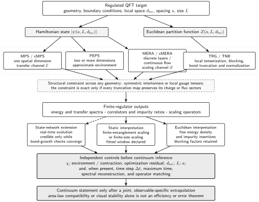
Real-time tensor evolution acts on a regulated state and adds step size, projection, maximum time, and spectral-window controls to the static bond, local-space, volume, and spacing limits. The diagram is schematic and makes no claim about present achievable times.

Exactly solvable two-site entanglement-growth fixture

Let

$$H=J\,X_1X_2, \qquad |\psi(0)\rangle=|00\rangle.$$

Because $(X_1X_2)^2=I$,

$$|\psi(t)\rangle =\cos(Jt)|00\rangle-i\sin(Jt)|11\rangle.$$

The exact observables and Schmidt values are

$$P_{11}(t)=\sin^2(Jt), \qquad \langle Z_1(t)\rangle=\cos(2Jt), \qquad \lambda_{1,2}=|\cos Jt|,|\sin Jt|.$$

A single two-site gate has no Trotter error, yet a bond-$1$ projection fails for generic $t$ because the exact state has Schmidt rank two. Thus a time-step scan alone can converge perfectly to the wrong projected dynamics. At $Jt=\pi/4$, both Schmidt values are $1/\sqrt2$ and the best bond-$1$ fidelity is only $1/2$.

Entanglement sets a credibility horizon

If the bipartite entropy reaches $S(t)$, an MPS across that cut needs at least

$$\chi(t)\geq e^{S(t)}$$

to represent the Schmidt spectrum without further assumptions. After many global quenches $S(t)$ grows approximately linearly over an intermediate regime, which implies rapidly increasing bond requirements; this behavior is not universal for every initial state or Hamiltonian. The credible time $t_*$ must therefore be defined from the observable:

$$t_*(\varepsilon)=\sup\left\{t: |O_{\chi',\Delta t',d'_{\rm loc},L'}(t)- O_{\chi,\Delta t,d_{\rm loc},L}(t)|<\varepsilon \ \text{for all prescribed refinements}\right\}.$$

Conserved energy, charge, or norm are necessary checks but can be exactly preserved by a projected method while an unconserved correlator drifts. A held-out local or nonlocal observable is required.

The joint control diagram shows how time-step and projection errors join the static axes. Inspect the false-plateau box: stable early-time data do not license a later interval.

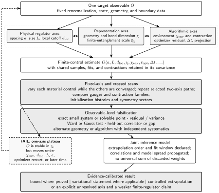
The reliable time window is observable specific and defined by joint refinement, conservation tests, and held-out comparisons. The schematic map rejects additive discarded-weight error bars and any extension beyond the first unresolved control.

Response, spectra, and scattering handoff

A regulated retarded correlator is

$$G_R(t,x)=-i\theta(t)\langle[O(t,x),O(0,0)]\rangle.$$

Its finite-time Fourier transform is convolved with the chosen window. Frequency resolution $\Delta\omega\sim2\pi/t_{\max}$ and window side lobes are reconstruction effects, not Hamiltonian errors. Report the raw time trace and covariance before a spectral model. For scattering or current matrix elements, the operator must be matched at each $a$, finite-volume propagation and boundary reflections must be excluded, and the final amplitude extraction follows the Hamiltonian observable route. Nonequilibrium interpretation belongs to the thermal and nonequilibrium volume.

The chapter’s tensor-network regulator and error record specifies the time, bond, operator, and claim fields that must accompany the trace.

Any real-time implementation must publish its convergence-defined time window; comparative time reach remains a dated Research question.

Adversarial failure: exact energy, wrong correlator

A fixed-bond TDVP evolution can preserve norm and energy to numerical precision because it follows a Hamiltonian flow inside the variational manifold. Once the exact state leaves that manifold, a retarded correlator may still drift badly. Compare increasing $\chi$, a two-site or Krylov evolution, and an exact small-volume trace; energy conservation alone cannot define $t_*$.

Observable-level validation checklist

• Reproduce the two-site fixture and an exact small-volume evolution.
• Scan $\Delta t$ or integrator tolerance at several fixed bond dimensions.
• Scan $\chi$ and projection thresholds at fixed time-step control.
• Monitor norm, energy, exact charges, local residuals, and discarded spectra.
• Vary $d_{\rm loc}$ for bosonic or link variables and $L$ before boundary signals arrive.
• Define $t_*$ from the target observable and all prescribed refinements.
• Report Fourier window, maximum time, frequency resolution, and reconstruction variation.
• Match currents or composite operators and keep the spacing limit separate.
• Route dated method reach to the Research methods dossier, not into a durable algorithm claim.

What you should be able to do

After this page, you should be able to:

1. construct a real-time tensor-network error analysis separating integrator, projection, bond, volume, local-space, spacing, and spectral-window effects; and
2. set a maximum credible time for a stated correlator from refinement and conservation tests rather than visual smoothness.

Exercises

1. Bond threshold. In the two-site fixture, at what earliest positive time does the smaller Schmidt probability reach $1/4$?

Solution

For $0\leq Jt\leq\pi/4$, the smaller probability is $\sin^2(Jt)$. Setting it to $1/4$ gives $Jt=\pi/6$, so $t=\pi/(6|J|)$.

2. Product-formula scaling. Halving $\Delta t$ changes an observable by $3\times10^{-4}$ in a second-order TEBD run, but doubling $\chi$ changes it by $2\times10^{-2}$. Which control dominates?

Solution

Bond or projection control dominates at that time. A smaller time step cannot justify more digits until the $\chi$ dependence is reduced or included explicitly in the error statement.

References

• Haegeman, Jutho, J. Ignacio Cirac, Tobias J. Osborne, Iztok Pižorn, Henri Verschelde, and Frank Verstraete. “Time-Dependent Variational Principle for Quantum Lattices.” Physical Review Letters 107 (2011): 070601. DOI.
• Paeckel, Sebastian, Thomas Köhler, Andreas Swoboda, Salvatore R. Manmana, Ulrich Schollwöck, and Claudius Hubig. “Time-Evolution Methods for Matrix-Product States.” Annals of Physics 411 (2019): 167998. DOI.
• Vidal, Guifré. “Efficient Simulation of One-Dimensional Quantum Many-Body Systems.” Physical Review Letters 93 (2004): 040502. DOI.