

Operator Bases, Effective Masses, and Excited-State Control
A finite operator basis supplies only as many independent operator-space directions as its overlap matrix supports. Effective-energy plateaus are useful diagnostics, but level isolation requires operators with the correct lattice quantum numbers, a well-conditioned correlation matrix, a generalized eigenvalue or explicitly modeled multi-state analysis, and stability under changes of basis, reference time, fit window, covariance treatment, and spectral model. A level label is credible only when these tests agree.
Required background. Euclidean Correlators and Spectral Information derives the finite-volume spectral matrix and boundary terms used here.
Helpful background. Normal Forms, Spectra, and Projectors reviews matrix spectral structure. Spectral Decomposition of Two-Point Functions supplies the Hilbert-space interpretation.
In the chapter’s observable-chain table, this page resolves the state-isolation stage: its output is a stable energy-and-overlap model, not yet a bare matrix element.
Operator bases define what can be resolved
Section titled “Operator bases define what can be resolved”For interpolating operators in one exact lattice-symmetry sector,
in the zero-temperature forward-propagation limit. Collect the first overlap vectors into the matrix . If , an operator-space analysis cannot produce independent principal correlators or determine independent overlap directions. More time slices do not create those missing directions.
This rank statement must not be confused with time-model identifiability. Even one exact scalar correlator can contain several exponential rates, and sufficiently many noiseless time samples can determine them under a finite-exponential ansatz. That recovery relies on a restrictive temporal model and can be extremely ill-conditioned in noise; it does not manufacture a second GEVP eigenvector or an independently normalized overlap vector.
Operators should differ in physical structure—spatial profile, derivative content, multi-particle construction, or displacement—not merely by overall normalization. Smearing changes overlaps and sometimes the regulator-level operator definition; its kernel, radius in physical units, iteration count, gauge transport, and ensemble dependence must be declared.
Basis and normalization conventions. Operators are projected into exact lattice irreducible representations and momenta before the matrix is formed. This page absorbs optional factors into and uses the site-wide conventions. Hermitian conjugation, reflection parity, smearing transformations, and vacuum subtraction remain local data.
At each positive time, an exact reflection-positive correlation matrix is Hermitian positive semidefinite. Estimated matrices can acquire small negative eigenvalues from noise. Large or persistent violations require investigation; blindly clipping them changes the likelihood and can create artificial stability.
Generalized eigenvalue method
Section titled “Generalized eigenvalue method”Choose a reference time for which is positive definite on the retained numerical subspace. Solve
In an exactly -state, full-rank model,
The correlation-matrix variational construction was introduced into lattice spectroscopy by Michael 1985, pp. 58–76. Higher states generate corrections whose suppression depends on the gaps, , , and the particular estimator. Choosing too early leaves large omitted-state effects; choosing it too late makes noisy and ill-conditioned. The asymptotic correction bounds and favorable choices such as are derived under explicit spectral assumptions by Lüscher and Wolff 1990, §5 and refined by Blossier et al. 2009, §§2–3.
Define a principal effective energy by
It is a derived diagnostic. Eigenvectors can reorder near degeneracies, so levels should be tracked by overlap continuity, quantum numbers, and multi-time information rather than by sorting eigenvalues independently at each time.
Whitening and conditioning
Section titled “Whitening and conditioning”Diagonalize . In exact arithmetic, whitening gives
If is comparable to statistical or floating-point uncertainty, inverse square roots amplify noise. A retained-rank choice must therefore be based on uncertainty-aware singular values and tested across resamples. The discarded directions define a changed operator subspace; the resulting systematic is not eliminated by calling the cut numerical.
A useful exact fixture has three states and three operators,
With full-rank , the GEVP recovers all three energies exactly. Making two columns of proportional leaves the correlator positive but reduces its operator-space rank: the GEVP loses one independent principal correlator. The surviving scalar time dependence can still contain both exponentials, so a separate multi-exponential fit may recover both energies if the sampling and finite-state model are sufficient. Injecting rank loss tests the GEVP claim; clustered energies and noisy long-time data test the temporal fit claim.
The QFT.org 2026 Chapter 2 benchmark, validated snapshot realizes the two-state version of both tests. Its full-rank GEVP recovers the exact generalized eigenvalues; after the overlap columns are made proportional, the matrix rank is one while a four-sample Prony recurrence still recovers the two input energies and to floating-point accuracy.
Competing spectral descriptions
Section titled “Competing spectral descriptions”GEVP analysis and direct multi-exponential fitting use the same spectral content differently. A robust calculation compares several controlled descriptions:
- principal correlators fitted to one or more exponentials;
- simultaneous matrix fits with shared energies and overlap vectors;
- Bayesian multi-state fits with explicit prior sensitivity;
- matrix-pencil or Prony-like methods on synthetic and high-precision data; and
- summation or ratio observables only when their altered contamination is derived.
Direct multiple-exponential methods make the distinction concrete: they can extract several rates from one temporal signal when their model-order and conditioning tests succeed Romiti and Simula 2019, §§II–IV. Such success is evidence for the time model, not evidence that a rank-one operator basis has become rank two.
Adding states always improves the maximum likelihood in an unconstrained nested model. It does not prove those states are identified. Examine held-out times, posterior-prior contraction, parameter correlations, predictive residuals, and recovery on mock data whose gaps and overlaps resemble the measured problem.
The effective-energy curve can exhibit a false plateau when two excited-state terms partially cancel over a finite window. For
off-diagonal or subtracted observables may have . The derivative of the bracket can be small even though neither term is. Moving the fit window modestly may not reveal the cancellation; changing the operator basis changes and is the decisive test.
Level identity in finite volume
Section titled “Level identity in finite volume”Finite-volume eigenstates are classified by total momentum and lattice irreducible representation, not by continuum spin alone. Multi-hadron operators can be essential even when the desired state resembles a single particle, because the spectrum contains every state with the same exact quantum numbers. Omitting them can leave a stable eigenvalue that is nevertheless a distorted mixture.
Volume dependence, overlap patterns, and inclusion of operators with different expected state content help identify levels. Converting the resulting spectrum into scattering amplitudes is a separate step governed by Spectra from Euclidean Correlation Matrices and the rest of Chapter 7.
Adversarial failure cases
Section titled “Adversarial failure cases”Rank-one basis for two nearby states. It cannot establish two independent GEVP levels or overlap directions. A multi-exponential fit to its time dependence is a separate, model-dependent route and must demonstrate model order, conditioning, and mock-data recovery.
GEVP reference time selected after viewing the answer. Scanning is a legitimate stability test; selecting one value without propagating the choice is not.
Eigenvalues sorted at every time. Near a crossing, this can splice two physical levels into one smooth-looking curve. Track eigenvectors and overlaps.
Covariance regularization hidden. Dropping small covariance eigenmodes changes the metric in data space. Report the retained modes and repeat the fit under justified variations.
Plateau agreement across operators that share the same smearing. Their excited-state overlaps may be strongly correlated. A structurally different operator gives a more independent test.
The shared inference map shows exactly where operator-basis rank and spectral model choice enter. Follow the discrete-level branch to see that a GEVP or multi-state fit produces finite-volume energies and overlaps, not yet a renormalized continuum observable.
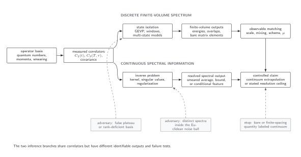
Two inference problems share the same regulated correlators. Discrete energies and overlaps, together with validated connected and disconnected three-point estimators, support bare matrix elements that require matching and continuum control before becoming physical results. Continuous reconstruction identifies only smeared averages, bounds, or conditional features at the demonstrated resolution; without separate matching and continuum analysis it ends at a methodological ceiling. Dashed boxes mark failure tests. The diagram is schematic and not to scale.
Observable-level validation checklist
Section titled “Observable-level validation checklist”Before assigning a finite-volume level, require:
- exact lattice quantum numbers and momentum for every operator;
- a declared smearing or displacement transformation with physical scale;
- Hermiticity and positive-semidefinite checks on ;
- uncertainty-aware rank and condition-number studies;
- variation of operator subsets, , fit windows, and state counts;
- level tracking by eigenvectors or overlaps, not time-local sorting;
- covariance treatment repeated through every resample;
- mock-data recovery including near-degeneracy and rank-loss failures; and
- held-out times or observables that were not used to select the model.
A useful exact fixture for these positive and negative tests uses three states and three operators.
Exercises
Section titled “Exercises”1. Exact GEVP. Let with square invertible and . Show that the generalized eigenvalues of are .
Solution
Multiply the GEVP by on the left and write . It becomes , which is diagonal. Each basis vector gives .
2. Rank-loss diagnostic. For two operators and two states, let the overlap columns be and . Show that has rank one for every . What information is lost to a GEVP, and what spectral information can remain in the scalar time dependence?
Solution
which is one outer product times a scalar. No choice of can create a second generalized eigenvector. A second independent operator structure is required.
The GEVP therefore cannot return two independent principal correlators or two overlap directions. Nevertheless, the scalar coefficient is a sum of and . With sufficiently many exact samples and a justified two-exponential ansatz, a temporal method can still determine both rates; finite precision and noise can make that inverse problem unstable.
What you can now do
Section titled “What you can now do”You should now be able to construct and condition a two-point correlation matrix, solve and test a GEVP, and reject a level claim that depends on one basis, window, or spectral model. Continue with Three-Point Functions, Matrix Elements, and Disconnected Contributions to extract a bare operator insertion while carrying the state-isolation problem into both source and sink channels.
References
Section titled “References”- Blossier, Benoît, Michele Della Morte, Georg von Hippel, Tereza Mendes, and Rainer Sommer. “On the Generalized Eigenvalue Method for Energies and Matrix Elements in Lattice Field Theory.” Journal of High Energy Physics 2009, no. 04 (2009): 094. doi:10.1088/1126-6708/2009/04/094.
- Lüscher, Martin, and Ulli Wolff. “How to Calculate the Elastic Scattering Matrix in Two-Dimensional Quantum Field Theories by Numerical Simulation.” Nuclear Physics B 339, no. 1 (1990): 222–252. doi:10.1016/0550-3213(90)90540-T.
- Michael, Christopher. “Adjoint Sources in Lattice Gauge Theory.” Nuclear Physics B 259, no. 1 (1985): 58–76. doi:10.1016/0550-3213(85)90297-4.
- QFT.org. “Lattice Observables and Continuum Inference Benchmark.” JavaScript source, validated 25 August 2026. SHA-256
d76924d8c724cb7c9307fb38265336495fa3ff1a98103b3fa4fa734262647c2a. Reproducibility record. - Romiti, Simone, and Silvano Simula. “Extraction of Multiple Exponential Signals from Lattice Correlation Functions.” Physical Review D 100, no. 5 (2019): 054515. doi:10.1103/PhysRevD.100.054515.