Regulated Hamiltonian Field Theory

A regulated Hamiltonian QFT is more than a finite matrix or a discretized energy density. It is a local algebra, a Hilbert-space representation and operator domain, a stable Hamiltonian, any exact constraints, boundary data, a class of states and observables, renormalization conditions, and an explicit path toward the continuum target. Separating these ingredients prevents numerical convergence within one regulator from being mistaken for convergence to a field theory.

Required background. Hamiltonian field theory supplies canonical initial data, and canonical quantization supplies the algebra–representation–state distinction.

Helpful background. Self-adjointness and unitary evolution clarify domain questions; lattice regulators clarify the target map.

The data that define the regulator

Regulator and domain card. Time is continuous and Lorentzian; space is a finite lattice of spacing $a$ and extent $L$ with declared boundaries. The algebra, Hilbert representation, domain, charge sector, and renormalized target are fixed before taking $a\to0$, $L\to\infty$, or any local-dimension or basis limit. A finite-dimensional Hamiltonian is Hermitian; an unbounded Hamiltonian requires a stated self-adjoint realization.

For a spatial lattice $\Lambda_a$ at fixed time, specify:

1. the local operator algebra and exact commutators;
2. the representation on $\mathcal H_{a,d}$, including any local cutoff $d$;
3. the dense domain $\mathcal D(H)$ for unbounded fields;
4. the Hamiltonian $H_{a,d}(\mathbf g)$ and boundary terms;
5. constraint generators and allowed boundary-charge sectors;
6. prepared states, observables, and their renormalization;
7. the tuning conditions and order of limits.

Hermiticity of a displayed expression is not automatically self-adjointness of an unbounded operator. On a finite tensor product with finite $d$, every Hermitian matrix is self-adjoint, but the $d\to\infty$ limit can still select a domain or extension. Stability also requires $H$ bounded below, uniformly enough for the intended limits.

Locality is regulator dependent. A finite-range spatial Hamiltonian is manifestly local on the lattice, while eliminating constraints or integrating out fields can produce nonlocal terms. The relevant test is whether physical propagation and commutators approach the target causal structure as the regulator is removed.

Continuum-targeted Hamiltonian algorithms likewise have to expose spatial, field-amplitude, volume, preparation, evolution, and measurement approximations rather than treating the finite Hamiltonian as the target itself Jordan, Lee, and Preskill 2012, pp. 1130–1133.

Free scalar chain as a complete example

For a real scalar in one spatial dimension, rescale the continuum field so that $[\phi_j,\pi_k]=i\delta_{jk}$. A periodic $N$-site Hamiltonian is

$$H_a=\frac12\sum_{j=0}^{N-1} \left[\pi_j^2+m_0^2\phi_j^2+\frac{(\phi_{j+1}-\phi_j)^2}{a^2}\right], \qquad L=Na.$$

With

$$\phi_j=\frac1{\sqrt N}\sum_p e^{ipx_j}\phi_p, \qquad p=\frac{2\pi n}{L},$$

the normal-mode frequencies are

$$\omega_a(p)^2=m_0^2+\widehat p^2, \qquad \widehat p=\frac2a\sin\frac{ap}{2}.$$

This verifies positivity for $m_0^2>0$, lattice translation invariance, and the continuum dispersion $\omega^2=m^2+p^2+O(a^2p^4)$. At fixed $L$, taking $a\to0$ increases $N$; taking $N\to\infty$ at fixed $a$ instead removes the volume cutoff but not the spacing cutoff.

If each oscillator is truncated to $d$ basis states, the projected matrices no longer satisfy $[\phi_j,\pi_j]=i$ exactly because a finite-dimensional trace of a commutator vanishes. Low-energy observables may converge with $d$, but that restoration must be demonstrated rather than assumed.

Physical constraints and evolution

For first-class regulated constraints $G_x$, consistency requires

$$[H,G_x]=0$$

or a declared covariant closure. Then exact time evolution preserves each charge sector. If a modified Hamiltonian has $[H_{\mathrm{app}},G_x]\ne0$, the leakage

$$\epsilon_G(t)=\sum_x \left\langle\bigl(G_x-q_x\bigr)^2\right\rangle_t$$

must be measured. A penalty $\lambda\sum_x(G_x-q_x)^2$ suppresses low-energy violations only as a function of $\lambda$ and the spectral couplings; finite $\lambda$ is not exact projection.

The shared diagram makes this distinction visible.

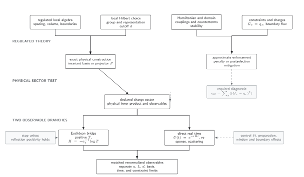
The Hamiltonian formulation separates local regularization, physical-sector construction, Euclidean transfer assumptions, and real-time evolution. Dashed stops mark penalty leakage and failure of reflection positivity; the diagram is schematic and not to scale.

Equal-time regulator comparison table

Axis	Finite definition	Quantity held fixed	Required test	Continuum role
Spatial lattice	spacing $a$, extent $L=Na$, boundaries	renormalized masses or ratios	dispersion and finite-volume sequences	$L\to\infty$, then or jointly $a\to0$
Local field space	amplitude, occupation, representation, or group cutoff $d$	matched low-energy couplings	commutator, symmetry, and observable convergence	$d\to\infty$ unless finite group is the target
Gauge sector	$G_x=q_x$, boundary flux	specified superselection sector	projector idempotence and $\epsilon_G$	exact before physical interpretation
Basis truncation	energy or conformal cutoff $\Lambda_B$	renormalization conditions	omitted-state and cutoff extrapolation	$\Lambda_B\to\infty$
Time evolution	formula and step $\delta t$	physical time and Hamiltonian	unitarity, conservation, step refinement	$\delta t\to0$ before long-time claim
Observation window	duration $T$ and sampling cadence	target resolution	window and boundary variation	$T\to\infty$ only when asymptotic quantity requires it
Cross-validation	matched operator, scale, scheme	same continuum target	Euclidean spectral and Ward comparisons	discrepancies vanish within combined errors

The light-front chapter supplies the complementary longitudinal, zero-mode, and harmonic-resolution entries. Equal-time and light-front finite boxes are distinct regulators even when both target the same continuum observable.

Regulator-removal contract

For each result, list the bare parameters as functions of the cutoffs, the renormalized conditions used to tune them, and a model for residual errors. A useful schematic form is

$$O=O_\star+c_a(a\Lambda)^p+c_Le^{-mL}+c_dd^{-\alpha} +c_t\delta t^r+c_TT^{-\gamma}+\cdots.$$

The powers are not universal and need theoretical or empirical support. Varying all cutoffs along one diagonal sequence can hide compensating errors; Cartesian or partially crossed studies are much more diagnostic.

Adversarial failure case

Suppose the oscillator basis frequency $\Omega(a)$ and dimension $d(a)$ are retuned at every spacing so that the lowest gap agrees with a target value. The gap can then look perfectly converged while the projected canonical-commutator residual $\epsilon_{\mathrm{CCR}}$, the cutoff-edge occupation, and $\langle1\lvert\phi\vert0\rangle$ drift in compensating directions. This sequence has fitted away one diagnostic rather than removed the regulator. Hold $\Omega$ fixed in one scan, vary $d$ independently at several $a$, and reserve a matrix element or unequal-time correlator that was not used in the tuning.

Observable-level validation

• Reproduce the free-chain dispersion and one equal-time covariance at fixed $(a,L)$ before turning on interactions.
• Verify the Hamiltonian’s lower bound or finite-volume low spectrum and state the self-adjoint domain when local operators are unbounded.
• Measure each exact charge and constraint through a squared residual, not only its expectation value.
• Vary $d$, $\Lambda_B$, $\delta t$, $L$, and $a$ independently enough to identify which axis moves the chosen spectrum or matrix element.
• Predict at least one held-out observable or regulator point with the same tuned couplings and error model.

Common pitfalls

Calling finite dimension a harmless implementation detail. It changes the local algebra unless the target itself has finite local Hilbert space. Demonstrate restoration in the states and observables used.

Checking energy conservation only. A method can conserve an approximate Hamiltonian while violating Gauss’s law or the target operator algebra. Monitor each exact structure independently.

Taking a thermodynamic limit at fixed bare parameters. Parameter tuning and volume removal answer different questions. State which renormalized quantities define the line of constant physics.

Learning outcomes

• Given a candidate regulated Hamiltonian, produce a specification separating its algebra, representation, domain, constraints, state, observables, boundary data, tuning conditions, and limit order.
• Given two apparently convergent cutoff sequences, design a crossed regulator study and a held-out observable that can distinguish genuine continuum convergence from compensation between errors.

Exercises

1. Expand $\widehat p^2$ through $O(a^2)$ and identify the leading dispersion artifact.

Solution

$\widehat p=p-a^2p^3/24+\cdots$, so $\widehat p^2=p^2-a^2p^4/12+O(a^4p^6)$.

2. Prove that finite-dimensional matrices cannot satisfy $[Q,P]=iI$ exactly.

Solution

The trace of any finite-dimensional commutator is zero by cyclicity, whereas $\operatorname{tr}(iI)=id\ne0$.

References

• Jordan, S. P., Lee, K. S. M., and Preskill, J. (2012). Quantum algorithms for quantum field theories. Science, 336, 1130–1133. DOI.

Further reading

• Kogut, J. B., and Susskind, L. (1975). Hamiltonian formulation of Wilson’s lattice gauge theories. Physical Review D, 11, 395–408. DOI.
• Reed, M., and Simon, B. (1975). Methods of Modern Mathematical Physics II: Fourier Analysis, Self-Adjointness. Academic Press. Bibliographic record.