

Lefschetz Thimbles and Holomorphic Contour Flow
Lefschetz-thimble and holomorphic-flow methods deform a real integration cycle into complexified field space without changing the integral. Along an individual thimble the imaginary part of a holomorphic action is constant, but the complete answer may require several thimbles, and the tangent-space Jacobian supplies a residual phase. Correctness therefore rests on homology, singularity avoidance, saddle-sector completeness, residual reweighting, and mixing—not on a visibly narrow phase distribution alone.
Required background. Anatomy and severity of a sign problem supplies phase and overlap diagnostics. Complex saddles and Lefschetz thimbles supplies the saddle decomposition.
Helpful background. Laplace’s method and steepest descent supplies local saddle geometry. Stokes jumps and saddle dominance supplies parameter-dependent intersection data.
Holomorphic flow and exact contour identity
Section titled “Holomorphic flow and exact contour identity”Convention and regulator card. Start with a finite-dimensional lattice-regulated integral . Complexify to . The integrand and observable must be holomorphic in the swept region; determinant zeros, poles, logarithmic branches, and boundaries are tracked explicitly. Orientation and every Jacobian phase are retained.
The upward holomorphic gradient flow is
Along a trajectory,
so increases while is constant. The flowed manifold suppresses regions away from saddle basins. If the deformation remains in the same relative homology class and crosses no singularity,
Parameterizing introduces the tangent Jacobian :
The Jacobian obeys
Its determinant can be expensive and strongly fluctuating. Replacing by changes the contour measure.
Thimbles, intersection numbers, and Stokes jumps
Section titled “Thimbles, intersection numbers, and Stokes jumps”A critical point satisfies . Its downward thimble is the union of flows ending at under downward flow; the dual upward cycle determines the integer intersection number . Formally,
An individual thimble has constant action phase, but the tangent orientation still supplies a residual phase, and distinct thimbles interfere. The decomposition and its Stokes jumps are properties of the integration cycle and parameter path, not a license to retain only the dominant real-part saddle. The homological formulation is developed systematically in Witten 2011, §§3.1–3.3.
At a Stokes wall, upward and downward flows connect critical points with equal action phase. Intersection numbers can jump while the total integral remains analytic. Numerically, nearby modes can become separated by high barriers on the flowed manifold; a Markov chain may remain trapped in one mode even though the contour is formally complete.
Exact one-angle flow test
Section titled “Exact one-angle flow test”Use the entire integrand
over one period. Writing is convenient locally but introduces logarithmic singularities at zeros of ; a flow implementation must not cross them or silently change branches. The exact target remains
For several flow times , parameterize and evaluate
Correctness requires to remain constant within quadrature error, including its imaginary part. Track the minimum distance to integrand zeros, the phase of , and transitions between all modes. As grows, local phase fluctuations may shrink while barriers and Jacobian fluctuations grow; an optimal finite flow time is an algorithmic tradeoff, not a different exact theory.
A stringent negative control samples only the mode connected to one saddle and omits another nonzero intersection sector. The resulting estimate can have a residual phase near unity and tiny error bars while disagreeing with the Bessel answer. Restoring the missing sector, including its relative phase and normalization, must repair the result.
Initial thimble proposals in lattice field theory already emphasized the residual measure phase and its computational cost Cristoforetti, Di Renzo, and Scorzato 2012, § II.C.1, pp. 074506-13–074506-14. Subsequent success in a model or finite volume is evidence for that domain; it does not establish a single-thimble description of a different theory or across a Stokes region.
Correctness and sampling conditions
Section titled “Correctness and sampling conditions”- Analytic deformation: identify all singular sets and verify the flowed cycle never crosses them.
- Homology: determine contributing sectors or demonstrate continuous deformation from the original contour at the chosen finite flow time.
- Jacobian: compute or unbiasedly estimate its magnitude and phase; quantify approximation error.
- Residual reweighting: report the average residual phase and its volume/flow-time scaling.
- Multimodal sampling: show transitions or combine sector-restricted estimates with independently computed relative normalizations.
- Stokes tracking: follow parameter changes with sufficient resolution to detect changing saddle connections.
- Reference checks: reproduce exact finite integrals, zero-flow results, and sign-free limits.
Adversarial failure cases
Section titled “Adversarial failure cases”Single-thimble assumption by saddle dominance. The smallest saddle need not be the only nonzero intersection sector, and cancellations can make subdominant sectors essential. Compute intersection data or use finite flow continuously connected to the original cycle.
Residual phase dropped after it looks narrow. Even a narrow phase distribution can shift a ratio observable through covariance. Reweight with the full phase and report numerator–denominator covariance.
Mode freezing mistaken for precision. Within-mode autocorrelation can be short while between-mode tunneling is absent. Use tempered flow, mode-resolved runs, and exact relative weights.
Stokes crossing hidden by parameter continuation. Smoothly continuing one saddle branch can omit a changed intersection combination. Check upward cycles and compare against a contour-integral reference on both sides.
The correctness map below attaches the contour branch to its decisive topological data. Inspect the homology and residual-phase stops: saddle dominance, a smooth flowed manifold, or a stable Monte Carlo history cannot replace intersection numbers and complete contour accounting.
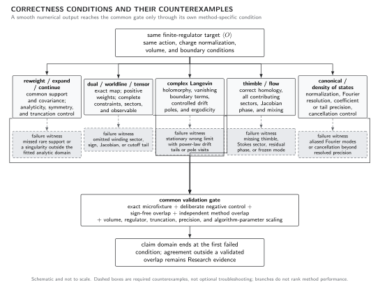
Each reformulation has a different correctness condition and a characteristic counterexample. Apparent numerical convergence is insufficient when overlap is absent, a dual sector or Jacobian is missing, complex-Langevin boundary terms survive, a contributing thimble is omitted, or canonical and density-of-states cancellations exceed resolved precision. The map is schematic and does not rank current algorithms.
Observable-level validation checklist
Section titled “Observable-level validation checklist”- State the original cycle, flow equation, action branch, singular sets, flow time, and Jacobian algorithm.
- Verify zero-flow recovery and flow-time invariance for the full complex integral.
- Report all identified saddle sectors, intersection evidence, mode transitions, and relative normalizations.
- Measure residual-phase and Jacobian distributions for the actual observable and versus volume.
- Reproduce an exact fixture and a deliberate missing-thimble or trapped-mode failure.
- Treat continuum and large-volume reach as Research evidence until the same checks survive those limits.
Exercises
Section titled “Exercises”1. Constant action phase
Section titled “1. Constant action phase”Show that upward holomorphic flow leaves constant.
Solution
Using the flow equation,
which is real and nonnegative. Hence and .
2. Why the Jacobian phase matters
Section titled “2. Why the Jacobian phase matters”Let a one-dimensional contour be . Compute its Jacobian and identify the residual phase.
Solution
. Thus
Even if were constant, this orientation phase fluctuates. Dropping it changes the contour integral.
Learning outcomes
Section titled “Learning outcomes”After working this page, you should be able to:
- Evolve a regulated contour and its tangent Jacobian, verify flow-time invariance, and compute the full residual phase.
- Diagnose a wrong result caused by a missing thimble, Stokes jump, residual-phase omission, or multimodal trapping using an exact contour benchmark.
Related topics
Section titled “Related topics”Canonical and density-of-states methods reorganize cancellations algebraically rather than geometrically. The finite-density method reliability matrix requires thimble evidence to overlap an independent method before extending a claim.
References
Section titled “References”- Cristoforetti, Marco, Francesco Di Renzo, and Luigi Scorzato. “New Approach to the Sign Problem in Quantum Field Theories: High Density QCD on a Lefschetz Thimble.” Physical Review D 86 (2012): 074506. doi:10.1103/PhysRevD.86.074506.
- Witten, Edward. “Analytic Continuation of Chern–Simons Theory.” In Chern–Simons Gauge Theory: 20 Years After, AMS/IP Studies in Advanced Mathematics 50 (2011): 347–446. doi:10.1090/amsip/050/19.