Finite-Volume Matrix Elements and 1→2 Transitions

A unit-normalized finite-volume matrix element is not yet an infinite-volume transition amplitude. The conversion multiplies by the density of final two-particle states—or, in the general formulation, by the residue of the same quantization matrix that produced the level—and by the finite-to-relativistic normalization of every stable one-particle state. The current must also be renormalized, and spectrum, current, and amplitude-parametrization uncertainties must be propagated together. Omitting a derivative or a factor $2EL^3$ changes the physical normalization, not merely a convention label.

Required background. Elastic Two-Body Quantization Conditions supplies the level density and determinant. Three-Point Functions, Matrix Elements, and Disconnected Contributions supplies bare Euclidean extraction and current renormalization. Form Factors and Local Operator Insertions supplies the infinite-volume amplitude conventions.

Helpful background. Scattering Amplitudes and Resonance Poles from Finite-Volume Spectra supplies the amplitude parametrization that enters the residue.

State normalization and the one-particle check

Let finite-volume momentum eigenstates have unit norm and infinite-volume one-particle states have relativistic norm:

$$\begin{aligned} \langle\mathbf p',L\vert\mathbf p,L\rangle &=\delta_{\mathbf p'\mathbf p},\\ \langle\mathbf p'\vert\mathbf p\rangle &=2E_{\mathbf p}(2\pi)^3 \delta^{(3)}(\mathbf p'-\mathbf p). \end{aligned}$$

On the finite momentum grid, $(2\pi)^3\delta^{(3)}(\mathbf p'-\mathbf p) =L^3\delta_{\mathbf p'\mathbf p}$, hence

$$\lvert\mathbf p\rangle =\sqrt{2E_{\mathbf p}L^3}\, \lvert\mathbf p,L\rangle.$$

Matrix-element normalization convention. Finite-volume eigenstates have unit norm, asymptotic one-particle states have relativistic norm, and the residue factor must use the same current, amplitude, and quantization-matrix conventions as the spectrum analysis.

The detailed choices are:

Field	Choice used on this page
Finite states	Unit normalized in a fixed $\mathbf P,\Lambda,\mu$ sector
Infinite one-particle states	Relativistic normalization $2E(2\pi)^3\delta^{(3)}$
Infinite two-particle state	One-channel benchmark uses an outgoing energy-normalized partial-wave state, $\langle E',\mathrm{out}\vert E,\mathrm{out}\rangle=\delta(E'-E)$
Current	$J_R(\mu)=Z_J(\mu,a)[J_{\rm bare}+\text{mixing and improvement terms}]$ in a declared scheme; the local insertion $J_R(0)$ is used below
Quantization branch	$\delta(E)+\phi(E,L)=n\pi$ with the branch $n$ unwrapped continuously
Generalization	Channel, spin, irrep, and partial-wave indices are retained in the quantization residue; the scalar formula is not applied componentwise to a coupled system

For a stable one-to-one transition at fixed allowed momenta, the normalization round trip is

$$\langle\mathbf p_f\vert J_R(0)\vert\mathbf p_i\rangle =\sqrt{2E_fL^3}\sqrt{2E_iL^3} \,\langle\mathbf p_f,L\vert J_R(0)\vert\mathbf p_i,L\rangle +O(e^{-m_{\rm gap}L}).$$

This free stable-particle limit is the first test of any code that later applies a two-particle residue factor.

The one-channel density-of-states factor

For one elastic partial wave, define the level-counting function

$$n(E,L)=\frac{\delta(E)+\phi(E,L)}{\pi}.$$

Near a simple level,

$$\rho_L(E_n) \equiv\frac{\mathrm dn}{\mathrm dE}\bigg\vert_{E_n} =\frac1\pi \frac{\partial}{\partial E} \left[\delta(E)+\phi(E,L)\right]_{E_n}.$$

Discretizing an energy-normalized scattering state gives

$$\lvert E_n,\mathrm{out}\rangle =\sqrt{\rho_L(E_n)}\,\lvert n,L\rangle.$$

Let

$$M_n^L =\langle n,L\vert J_R(0)\vert\mathbf p_i,L\rangle, \qquad \mathcal H(E_n) =\langle E_n,\mathrm{out}\vert J_R(0)\vert\mathbf p_i\rangle.$$

The conversion in these explicitly chosen normalizations is

$$\boxed{ \left\lvert\mathcal H(E_n)\right\rvert^2 =2E_iL^3\,\rho_L(E_n) \left\lvert M_n^L\right\rvert^2 =\frac{2E_iL^3}{\pi} \frac{\partial(\delta+\phi)}{\partial E}\bigg\vert_{E_n} \left\lvert M_n^L\right\rvert^2.}$$

The box emphasizes one normalization benchmark, not a universal scalar formula. If the current is spatially integrated, if the final state is momentum-normalized, or if identical-particle factors are placed elsewhere, explicit powers of $L$, $2E$, and phase space move. The invariant round trip is to convert back and recover $M_n^L$ with the same definitions.

In the noninteracting limit $\delta=0$, the derivative of $\phi$ is exactly the free level density. Near a narrow elastic resonance, $\partial_E\delta$ can be large; setting $\delta'=0$ therefore fails precisely where final-state interactions matter most. The original weak-decay relation and its normalization logic were established by Lellouch and Lüscher 2001, §§ 2–4, pp. 33–41.

Matrix residue for mixed partial waves and channels

Write the quantization matrix in an ordered basis as

$$Q(E)=\mathcal K^{-1}(E)+F(E,\mathbf P,L), \qquad Q(E_n)v_n=0.$$

For a simple root and $v_n^\dagger v_n=1$, its pole residue is

$$\mathcal R_n =\lim_{E\to E_n}(E-E_n)Q(E)^{-1} =\frac{v_nv_n^\dagger} {v_n^\dagger[\partial_EQ(E_n)]v_n}.$$

A vector $\mathcal H$ of infinite-volume transition amplitudes in the same channel–partial-wave basis is contracted with $\mathcal R_n$. The precise master equation depends on whether kinematic factors are included in $\mathcal H$, $F$, and the finite-volume current projection; it must be fixed by matching its one-channel reduction to the boxed density formula. This residue construction, including multichannel and arbitrary injected momentum, is derived by Briceño, Hansen, and Walker-Loud 2015, §§ II–IV and generalized for arbitrary spin by Briceño and Hansen 2015, §§ II–III.

The residue makes three facts visible:

• a finite-volume level constrains only the amplitude combination parallel to its null vector $v_n$;
• the derivative acts on the full energy dependence of both the scattering amplitude and finite-volume geometry; and
• a nearly degenerate or multiple root requires a subspace treatment, not the simple rank-one formula.

A one-to-two amplitude in a coupled final state cannot be reconstructed from one matrix element. Multiple levels, irreps, current kinematics, and a bounded amplitude parametrization are needed to identify its components.

Joint covariance and a conversion contract

The spectrum and current matrix element usually come from the same gauge configurations and correlator analysis. Use a single outer resample to repeat:

1. two- and three-point correlator construction;
2. spectrum and overlap extraction;
3. current renormalization and improvement;
4. the correlated scattering-amplitude fit;
5. evaluation of $\partial_EQ$ or $\partial_E(\delta+\phi)$;
6. finite-to-infinite-volume conversion; and
7. any later analytic continuation or form-factor fit.

This preserves correlations among $E_n$, $M_n^L$, masses, scale, $Z_J$, and the amplitude derivative. Computing the factor only at central values and multiplying independent errors loses the largest correlation near a steep phase shift.

Adversarial failure. A calculation uses unit-normalized finite-volume states but compares $M_n^L$ directly with a relativistically normalized amplitude. Its values shrink with $L$ and are interpreted as a physical form-factor trend. The free one-to-one round trip exposes the missing $\sqrt{2EL^3}$ factors; the one-to-two case additionally exposes the missing level-density derivative.

The branch-status map places current insertions beside, not inside, the elastic spectrum branch. Inspect the separate current endpoint: residue normalization, operator matching, shared spectrum–matrix-element covariance, and held-out checks are additional evidence requirements.

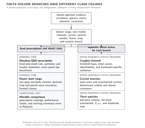
Finite-volume branches have different claim ceilings. A fixed massless-field prescription and an exact power-law test are durable; mutable prescription comparisons may move to Research. Coupled-channel, current-insertion, and three-particle claims require separate dated status and validation. The map is schematic and not to scale.

Observable-level validation

Before accepting a converted transition amplitude, verify that:

• the finite and infinite state norms, current Fourier projection, identical- particle factors, and current-renormalization scheme are explicit;
• the same branch and amplitude parametrization reproduce the level and its derivative factor;
• the one-to-one normalization and noninteracting two-particle density limit are recovered analytically;
• a multiple or nearly degenerate quantization root is treated as a subspace;
• one outer resampling chain propagates spectrum, current, $Z_J$, kinematic, and parametrization covariance; and
• alternative current improvement, partial-wave, channel, and amplitude forms are included when they move the observable.

What you can now do

You can now (1) convert a unit-normalized finite-volume matrix element to the stated energy-normalized one-to-two amplitude with every $2EL^3$ and derivative factor visible, and (2) propagate spectrum, current, renormalization, and amplitude-parametrization covariance through a noninteracting or synthetic round-trip test.

Coupled-Channel Quantization and Inference supplies the matrix amplitude entering $Q$. Physical electroweak and hadronic interpretation belongs to Gauge Theories and the Standard Model, and dated formalism status belongs to the Lattice and Hamiltonian Field Theory Research area.

Exercises

1. Derive the density factor. Starting from $\langle E'\vert E\rangle=\delta(E'-E)$ and level spacing $\Delta E=1/\rho_L$, derive $\lvert E_n\rangle=\sqrt{\rho_L}\lvert n,L\rangle$.

Solution

On the discrete grid, $\delta(E_n-E_m)\simeq\delta_{nm}/\Delta E =\rho_L\delta_{nm}$. Therefore $\sqrt{\rho_L}\lvert n,L\rangle$ has continuum norm $\delta(E_n-E_m)$. Equivalently, $\lvert n,L\rangle=\sqrt{\Delta E}\lvert E_n\rangle$.

2. Sensitivity near a resonance. If $\partial_E\delta$ doubles while all other quantities and $M_n^L$ are fixed, does $\lvert\mathcal H\rvert^2$ necessarily double?

Solution

No. It is proportional to $\partial_E\delta+\partial_E\phi$, so it doubles only if $\partial_E\phi$ is negligible. In an actual analysis the level position and $M_n^L$ also co-vary with the fitted phase shift, which is why joint resampling is required.

References

• Briceño, Raúl A., and Maxwell T. Hansen. “Multichannel 0→2 and 1→2 Transition Amplitudes for Arbitrary Spin Particles in a Finite Volume.” Physical Review D 92 (2015): 074509. DOI. Open PDF.
• Briceño, Raúl A., Maxwell T. Hansen, and André Walker-Loud. “Multichannel 1→2 Transition Amplitudes in a Finite Volume.” Physical Review D 91 (2015): 034501. DOI. Open PDF.
• Lellouch, Laurent, and Martin Lüscher. “Weak Transition Matrix Elements from Finite-Volume Correlation Functions.” Communications in Mathematical Physics 219 (2001): 31–44. DOI. Open PDF.