

Bare Parameters, Tuning Conditions, and Continuum Targets
A continuum trajectory is defined by renormalized conditions, not by holding bare couplings fixed while the lattice spacing changes. Let be the rank of the independent conditions needed to fix the target-defining relevant, marginally relevant, and exactly marginal data after exact symmetries and redundant directions are accounted for. At least independent physical inputs are then required to select the target theory. Scale setting converts dimensionless lattice results into units; an input may participate in a correlated global fit, but it cannot later be counted as an independent prediction. Only after this trajectory is established can Chapter 2 perform continuum inference for additional observables.
Required background. Lattice Regulators and Target Continuum Theories supplies the finite-regulator specification. Regulators, Cutoffs, and Continuum Limits supplies the general distinction between a bare family and a renormalized limit.
Helpful background. Critical Surfaces, Crossover, and Corrections to Scaling describes critical manifolds and corrections to scaling. Regulator Removal and Renormalized Predictions explains scheme-dependent coordinates and scheme-independent predictions.
Bare coordinates do not label a physical theory by themselves
Section titled “Bare coordinates do not label a physical theory by themselves”Let a regulated action depend on dimensionless bare coordinates
where , for a scalar quartic interaction, and more generally for an operator of engineering dimension . These powers make the coordinates dimensionless; near an interacting fixed point, RG relevance is instead determined by the eigenvalues of the linearized flow, including anomalous dimensions and operator mixing. A change in generally changes the values of needed to describe the same renormalized physics.
A continuum target is specified by renormalized conditions
where each is a dimensionless observable or a dimensionless ratio constructed from a renormalized quantity. Solving these equations at each defines a trajectory
At fixed physical volume, a target observable is then predicted rather than tuned:
with the volume prescription explicit. On an anisotropic lattice, the corresponding condition is in each direction. A declared joint path may instead use , but it is a different prescription. A fit of before establishing that the remain fixed mixes cutoff effects with a drift through theory space.
Tuning and scheme conventions. This page uses Euclidean lattice variables and the site-wide conventions. The renormalization scheme, scale , finite-volume condition, boundary data, and definitions of every are local. Bare coordinates may be convenient simulation inputs; they are not physical observables. A “line of constant physics” means a trajectory satisfying declared renormalized conditions within quantified tolerances.
The rank is not obtained by merely counting every coupling with a nonnegative engineering dimension. Each independent relevant scaling field must be fixed or tuned. An exactly marginal field labels a family of continuum theories and must be specified when it is part of the target; a marginally relevant field needs boundary data or an equivalent generated scale. A marginally irrelevant field normally flows to the fixed point without an independent tuning condition. Symmetries can forbid fields, redundant operators do not add physical inputs, and parameters intentionally varied across a family are specified rather than tuned to one value. This critical-surface interpretation follows Wilson 1971, pp. 3181–3182 and the review by Wilson and Kogut 1974, pp. 75–199. Breaking a target symmetry can allow new relevant terms and enlarge the tuning problem. This is why the classification on Exact Symmetries, Broken Spacetime Symmetries, and Restoration precedes parameter tuning.
A free scalar tuning relation
Section titled “A free scalar tuning relation”The free theory provides an exact benchmark. For the nearest-neighbor scalar with on an isotropic lattice, the infinite-time momentum-space pole obeys
where is the pole mass extracted from exponential Euclidean-time decay. At finite periodic temporal extent, define as the transfer gap: it obeys the same relation, while the correlator is exactly a forward-plus-backward image, or cosh, form rather than a single exponential. To hold the physical pole mass fixed as changes, the bare mass must follow
Holding instead gives
so the measured pole mass is shifted downward by . The shift vanishes in the continuum limit, but its sign and coefficient provide a clean test that tuning code distinguishes a bare parameter from the measured mass.
Suppose the continuum step is taken at fixed physical volume . Then must increase as decreases. A valid three-spacing sequence might use
with set by the exact hyperbolic-sine relation at each row. The equal values of separate cutoff changes from volume changes. A separate volume study at fixed , such as , diagnoses periodic images.
For an interacting scalar, one condition for the mass is insufficient if the renormalized coupling is also part of the target. A second condition can be defined through a connected four-point function, finite-volume scattering observable, or other dimensionless renormalized coupling. Its scheme and kinematics must be named. Different legitimate definitions yield different bare trajectories at finite ; provided the continuum limits exist and both trajectories enter the same universality class, their predictions agree after scheme translation and matching.
Scale setting without circularity
Section titled “Scale setting without circularity”Lattice calculations first produce dimensionless quantities such as and ratios . To express a dimensionful answer, choose a reference quantity of nonzero mass dimension with known or conventionally assigned physical value and determine
For a reference mass this reduces to . For a reference length or flow time it gives, respectively,
The choice of is part of the analysis. If is also used to set the scale, agreement for in physical units is an input, not an independent test. A clean design declares the roles of:
- tuning observables, which choose the bare trajectory;
- the scale-setting observable, which assigns units;
- validation observables, whose independent information is withheld from the defining conditions; and
- target observables, whose continuum values answer the scientific question.
These roles need not correspond to disjoint data files: a correlated global fit can determine tuning, scale, and target quantities jointly. What matters is that an input is not relabeled as a held-out prediction and that all shared covariance is retained. In a theory studied for its internal continuum limit rather than phenomenology, one may set units by a mass gap, gradient-flow scale, or finite-volume reference and quote all other results as dimensionless ratios. No choice removes the need to propagate the reference uncertainty and its correlations.
Circularity can also be subtler. If the same fitted correlator supplies both , an operator renormalization, and the final matrix element, their statistical and model uncertainties are correlated. Treating them as independent can make a tuned trajectory look artificially precise. Preserve statistical correlations with a joint likelihood or by repeating the complete tuning–scale–matching–target pipeline inside every bootstrap or jackknife sample. Cross-covariances from shared ensembles, scale inputs, renormalization factors, and bare-parameter interpolation belong to the result. Correlated model systematics additionally require shared nuisance parameters, coherent fit variations, or model averaging; resampling alone does not supply them.
The order of limits is part of the target
Section titled “The order of limits is part of the target”Write a full target statement as an iterated or joint limit. For a massive zero-temperature observable one possible order is
The inner limit holds physical , the renormalized conditions, the operator scheme, and the target kinematics fixed. The outer limit removes the finite box. A simultaneous trajectory can be used only if the target data remain matched while and , and if mixed cutoff–volume terms are included in the error model. If the define a finite-volume scheme, changing requires the corresponding matching or retuning. The local effective-action basis that organizes the cutoff terms is developed by Symanzik 1983, Part I, §§2–4. The trajectory should not be denoted by a single unlabeled arrow.
Other questions require a different order:
- a thermal continuum limit takes and at fixed and fixed physical spatial volume, followed by a thermodynamic limit or a declared joint path;
- a critical continuum limit tunes the correlation length in lattice units to infinity while maintaining the desired physical normalization;
- in a broken phase, the state-selecting order can differ from the reversed chiral and thermodynamic limits; and
- as an analysis order, scattering amplitudes require finite-volume spectral extraction before an infinite-volume amplitude interpretation.
These are changes of scientific question, not preferences in numerical sequencing.
The complete observable chain is shown below. Inspect the separation among tuning, operator matching, scale setting, and extrapolation; none can be inferred from a small statistical error bar in the previous stage.
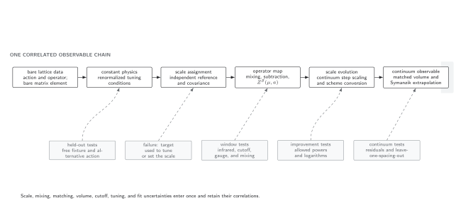
A continuum prediction requires a tuned bare trajectory, a regulator-consistent calculation, and a renormalized observable in a named scheme. When momentum-space lattice perturbation theory is used, its propagators, vertices, and Brillouin zone must be retained unless a controlled matching or subtraction justifies a continuum replacement. Step scaling or scheme conversion is optional when the matching scale is already suitable. The failure exits reject an untuned trajectory, an unjustified continuum propagator inside a lattice loop, a defining input counted as a prediction, and a one-spacing or unsupported extrapolation. Schematic, not to scale.
The order-of-limits map summarizes why a trajectory must declare more than . Follow each axis with its held-fixed quantities, and inspect the two crossed paths where an apparently familiar limit changes the physical target.
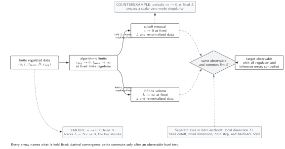
Both main routes apply cutoff removal and infinite volume while matching the target data before their results are compared. A broken phase and the periodic massless scalar give genuine order tests; at fixed site count is instead a misidentified path because the box shrinks. Other truncation and time-evolution axes need their own declared schedules. The diagram is schematic and not to scale.
Under-tuning and identifiability
Section titled “Under-tuning and identifiability”Let be the response matrix near a proposed trajectory. If lacks rank in the target-defining subspace, the chosen conditions do not determine all required directions. This can happen when two conditions are physically redundant, statistically indistinguishable, or insensitive to a breaking operator.
Useful diagnostics include:
- singular values of a dimensionless, covariance-weighted response matrix across the simulated region—the apparent conditioning otherwise depends on arbitrary parameter and observable normalizations;
- stability when one tuning observable is replaced by another;
- held-out quantities sensitive to each symmetry-breaking direction;
- priors or constraints stated explicitly rather than hidden in interpolation; and
- ensembles on both sides of the target so the solution is interpolated rather than extrapolated in bare space.
For example, after choosing a diagonal matrix of declared bare-parameter scales and a covariance matrix for the conditions, one may inspect the whitened response . Its singular values have a stated statistical metric; raw singular values of do not.
The opposite problem is overconstraining: more conditions than adjustable physical inputs need not agree at finite . Their mismatch can be valuable cutoff evidence. Fitting every condition exactly by adding arbitrary bare terms may change the regulator family rather than improve the original one.
Adversarial failure cases
Section titled “Adversarial failure cases”Bare couplings held fixed. A sequence at fixed generally changes renormalized masses and couplings. It is a scan through theories, not automatically a continuum trajectory.
One condition for two relevant directions. A precise mass match cannot also determine an independent interaction strength. The uncontrolled direction can drift while the mass stays fixed.
A scale input counted again as a prediction. If a target mass fixes , reproducing that mass in physical units is guaranteed. Validate using another dimensionless ratio or a genuinely held-out observable.
Continuum fit on a mistuned sequence. Smooth behavior does not show constant physics. Plot the tuning observables versus and propagate their residual deviations into .
Critical and infinite-volume limits exchanged silently. Finite volume rounds a phase transition and can remove spontaneous symmetry breaking. State which limit defines the target state.
A single action family. Agreement of several observables may still inherit the same matching or fit bias. A second discretization with a different artifact pattern is a stronger cross-check.
Observable-level validation checklist
Section titled “Observable-level validation checklist”The tuning and limit-order rows of the target and regulator table state the renormalized quantities held fixed and the regulator sequence needed to interpret a common continuum limit.
Before extrapolating a target quantity, require:
- the rank and RG character of the independent target-defining directions;
- enough independent renormalized conditions to fix that rank, or a proof that a condition is unnecessary;
- a response matrix with adequate rank and conditioning;
- ensembles bracketing the target conditions at every spacing;
- scale-setting, tuning, validation, and target information assigned declared roles, with no defining input counted as a held-out prediction;
- residual mistuning propagated with joint statistical covariance and coherent analysis-model variations;
- operator scheme, scale, mixing, and matching recorded before the fit;
- cutoff and finite-volume controls varied independently;
- an explicit order of limits with held-fixed quantities; and
- held-out observables or a second regulator confirming the target rather than defining it.
Chapter 2 develops the actual Lines of Constant Physics and Continuum Extrapolation and Scale Setting and Dimensionless Ratios workflows. The present page fixes their inputs and stop conditions.
Exercises
Section titled “Exercises”1. Exact free tuning. Expand the exact relation through . Then suppose one instead sets the bare parameter to . Expand the pole mass actually realized and determine its relative error.
Solution
The expansion is
Thus the correctly tuned bare ratio is . If one instead inserts into the pole equation,
Therefore
The naive choice makes the measured pole mass too small at leading order.
2. Detecting under-tuning. Two bare parameters are constrained by one condition . Show that the target is not unique and propose a second condition.
Solution
The solutions form the line ; the response matrix has rank one. Any observable sensitive to the orthogonal direction, for example , can serve as a second condition if it is a well-defined renormalized quantity. The pair has Jacobian determinant and locally determines both coordinates.
What you can now do
Section titled “What you can now do”You should now be able to define a target trajectory through bare-parameter space using independent renormalized conditions, expose under-tuning and circular scale setting, and state a physically meaningful order of limits. The next chapter, Lattice Observables and Continuum Inference, carries this specification through correlator analysis, operator renormalization, improvement, uncertainty propagation, and continuum extrapolation.
References
Section titled “References”- Symanzik, Kurt. “Continuum Limit and Improved Action in Lattice Theories. I. Principles and Theory.” Nuclear Physics B 226, no. 1 (1983): 187–204. doi:10.1016/0550-3213(83)90468-6.
- Wilson, Kenneth G. “Renormalization Group and Critical Phenomena. I. Renormalization Group and the Kadanoff Scaling Picture.” Physical Review B 4, no. 9 (1971): 3174–3183. doi:10.1103/PhysRevB.4.3174.
- Wilson, Kenneth G., and John Kogut. “The Renormalization Group and the Expansion.” Physics Reports 12, no. 2 (1974): 75–199. doi:10.1016/0370-1573(74)90023-4.
Further reading
Section titled “Further reading”- Lüscher, Martin. “Advanced Lattice QCD.” In Les Houches Summer School in Theoretical Physics, Session 68: Probing the Standard Model of Particle Interactions, 1998, pp. 229–280. arXiv:hep-lat/9802029.
- Montvay, István, and Gernot Münster. Quantum Fields on a Lattice. Cambridge University Press, 1994, chs. 3–5. doi:10.1017/CBO9780511470783.