Lattice Geometry, Boundaries, and Anisotropy

Lattice geometry is part of the theory’s finite-regulator definition, not an implementation detail. Spacings determine the ultraviolet cutoff and discrete derivative symbols; physical extents determine infrared resolution and periodic images; boundary conditions select the allowed modes and the state or ensemble; anisotropy changes the relation between spatial momentum and transfer energy. Changing any one of them can change the observable before a continuum limit is taken.

Required background. Lattice Regulators and Target Continuum Theories supplies the target–regulator–observable–limit specification used here.

Helpful background. Boundaries and State Preparation explains how Euclidean boundary data prepare states. Fourier Series, Fourier Transforms, and Plancherel Theory provides the transform identities behind the mode sets.

Cells, extents, and physical scales

For an orthogonal $d$-dimensional lattice, write

$$x_\mu=a_\mu n_\mu, \qquad n_\mu=0,\ldots,N_\mu-1, \qquad L_\mu=N_\mu a_\mu.$$

The tuple $(a_\mu,N_\mu)$ carries two logically distinct kinds of data. The spacing $a_\mu$ controls the largest resolvable momentum, while $L_\mu$ controls the smallest nonzero momentum and the separation from boundaries or periodic images. A continuum study therefore needs at least two dimensionless controls for every physical mass scale $m$:

$$am\quad\text{and}\quad mL.$$

Small $am$ does not imply large $mL$, and large $N=L/a$ does not establish either one without a physical scale. For several spacings or masses, replace these by a hierarchy such as

$$a\Lambda_{\mathrm{UV}}\ll1, \qquad m_{\mathrm{gap}}L\gg1, \qquad a\ll r\ll L,$$

where $r$ is the separation probed by a local correlator. Each inequality answers a different question: cutoff resolution, finite-volume suppression, and the existence of an intermediate physical window.

Geometry and conventions. This page uses a flat Euclidean orthogonal lattice, positive spacings $a_\mu$, and the site-wide natural-unit conventions. A direction called “time” is a distinguished Euclidean direction used for transfer and correlation functions; it is not a second Lorentzian signature. Boundary phases, cell placement, and anisotropy are declared locally.

Fields may live on sites, oriented links, plaquettes, or more general cells. Reversing an oriented link changes its group variable to the inverse in gauge theory; reversing a $p$-cell changes the sign of a cochain variable when orientation matters. Those facts become central in the gauge chapter. For the scalar benchmark, only site variables are required.

Boundary conditions select different finite theories

On a direction of length $L=Na$, a twisted boundary condition is

$$\phi(x+L\hat\mu)=e^{i\theta_\mu}\phi(x).$$

Its allowed momenta are

$$p_\mu=\frac{2\pi n_\mu+\theta_\mu}{L_\mu}, \qquad n_\mu\in\mathbb Z\pmod{N_\mu}.$$

Periodic fields have $\theta_\mu=0$ and include a zero mode. Antiperiodic fields have $\theta_\mu=\pi$ and exclude it in that direction. A general twist can give continuous access to shifted finite-volume momenta, but it changes winding contributions and must be applied consistently to every charged field and interaction. It is not merely a relabeling of the Fourier grid.

Open boundaries instead remove the identification of opposite faces. Translation invariance is lost, ordinary plane waves no longer diagonalize the kernel, and summation by parts leaves edge terms. For a one-dimensional forward difference,

$$(\nabla^+g)_n=\frac{g_{n+1}-g_n}{a},$$

one finds on sites $n=0,\ldots,N-1$

$$a\sum_{n=0}^{N-1} f_n(\nabla^+g)_n =-a\sum_{n=1}^{N-1}(\nabla^-f)_n g_n +f_{N-1}g_N-f_0g_0.$$

The endpoint values and which sites are dynamical determine the variational problem. Dropping the last two terms silently imposes a boundary condition. Dirichlet, Neumann, Robin, and dynamical boundary conditions correspond to different domains for the quadratic operator, so they can change spectra and correlation functions even at fixed bulk action.

For a massive theory with periodic boundaries, a local observable far from contact often receives image corrections of order $e^{-mL}$, up to powers of $mL$. Open boundaries instead produce position-dependent boundary contamination typically suppressed by the distance to the edge. Neither estimate applies unchanged to a massless field or a long-range force.

Anisotropy separates spatial and transfer scales

Let $a_t$ be the Euclidean-time spacing and $a_s$ the common spatial spacing. The free scalar action

$$S=\frac{a_ta_s^{d-1}}{2}\sum_x\left[ (\nabla_t^+\phi_x)^2 +\sum_{i=1}^{d-1}(\nabla_i^+\phi_x)^2 +m_0^2\phi_x^2 \right]$$

has kernel

$$K(p)=m_0^2 +\frac{4}{a_t^2}\sin^2\!\left(\frac{a_tp_0}{2}\right) +\frac{4}{a_s^2}\sum_i\sin^2\!\left(\frac{a_sp_i}{2}\right).$$

Analytically continue the Euclidean energy variable to a pole at $p_0=iE$. The dispersion relation is

$$\frac{4}{a_t^2}\sinh^2\!\left(\frac{a_tE}{2}\right) =m_0^2+\widehat{\mathbf p}^{2}_s, \qquad \widehat{\mathbf p}^{2}_s =\frac{4}{a_s^2}\sum_i\sin^2\!\left(\frac{a_sp_i}{2}\right).$$

This relation is exact for the free nearest-neighbor action. Its small-spacing limit is $E^2=m_0^2+\mathbf p^2$, but finite-spacing corrections depend separately on $a_tE$ and $a_sp_i$. An interacting anisotropic action generally has a renormalized anisotropy $\xi_R=a_s/a_t$ that differs from its bare input. One must determine $\xi_R$ from an observable—commonly a dispersion relation or matched spatial and temporal scales—before using it to convert time steps into spatial units Klassen 1998, §§2–4.

The geometry–dispersion map summarizes which features of this derivation change when the boundary phase, anisotropy, or zero-mode treatment changes. Inspect especially the distinction between the mode set, the difference-operator symbol, and the continuum expansion.

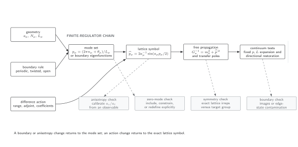
Geometry and action data jointly determine finite-regulator propagation. Periodic, twisted, open, and anisotropic choices cannot share one momentum or dispersion formula without translation. The continuum expansion is a tested limit, not an identification at finite spacing. Schematic, not to scale.

Periodic and open scalar correlators

For a periodic massive free scalar, the finite-volume correlator can be written either as a mode sum or an image sum. In one spatial dimension at equal Euclidean time,

$$G_L(x)=\frac1L\sum_{p=2\pi n/L} \frac{e^{ipx}}{2E(p)} =\sum_{\ell\in\mathbb Z}G_\infty(x+\ell L),$$

where the second equality follows from Poisson summation under the usual convergence assumptions. The closest nonzero images give the leading large-$mL$ correction. This representation provides an independent check of Fourier normalization: a missing factor of $L$ cannot satisfy both forms.

With Dirichlet boundaries at $x=0,L$, the normal modes are $\sin(n\pi x/L)$, $n\ge1$, and the correlator depends on $x$ and $y$ separately rather than only on $x-y$. There is no translation-invariant effective mass at all source positions. Reliable bulk extraction requires distances from each boundary large compared with the inverse gap, or an explicit boundary-state analysis.

The comparison exposes a useful principle: a boundary condition can be harmless for a sufficiently local bulk observable in a controlled large-volume limit while materially changing finite-volume spectra, zero modes, and state preparation. Whether it is harmless is an observable-level statement.

Limit order and near-miss cases

Fixed site count while $a\to0$. Since $L=Na$, the physical box shrinks. The highest momentum grows, but the lowest nonzero momentum grows too; no fixed infrared physics remains.

Thermal and vacuum limits. If the distinguished Euclidean-time extent is $\beta=1/T$, taking $N_t\to\infty$ at fixed $a_t$ sends $T\to0$ but does not remove the temporal cutoff. Taking $a_t\to0$ at fixed $N_t$ sends $T\to\infty$. A vacuum continuum limit needs both the physical temperature and the cutoff trajectory declared. Thermal phase structure belongs to Thermal and Nonequilibrium QFT.

Massless limit before infinite volume. A periodic scalar zero mode becomes singular at $m=0$ in finite volume. Taking $L\to\infty$ first for suitable local observables may give a different intermediate problem. A zero-mode prescription is part of the measure, not a numerical convenience.

Twisting only the valence observable. In a theory with dynamical charged fields, twisting the measured propagator but not the determinant or ensemble defines a partially twisted setup. It may be useful under stated hypotheses, but it is not identical to a fully twisted theory.

Using isotropic formulas after anisotropic tuning. A bare input $a_s/a_t$ is not automatically the physical anisotropy. Applying an isotropic dispersion formula can convert a calibration error into an apparent mass shift.

Observable-level validation checklist

For every geometry and boundary choice, verify:

• $N_\mu$, $a_\mu$, and $L_\mu=N_\mu a_\mu$ are mutually consistent and carry units;
• Fourier modes satisfy the declared boundary phase and the transform is complete;
• the action variation retains every open-boundary term;
• the constant mode is included, constrained, or removed by an explicitly stated definition;
• anisotropy is calibrated by a physical observable rather than assumed from a bare coefficient;
• cutoff and volume studies hold different dimensionless controls fixed;
• source and sink positions are varied to expose boundary contamination; and
• any exchange of $a\to0$, $L\to\infty$, $T\to0$, or $m\to0$ is tested on the same observable.

A numerical check of the periodic dispersion and image sum must use the analytic equalities above as its reference.

Exercises

1. Twisted momentum. Derive the allowed momenta for $\phi(x+L)=e^{i\theta}\phi(x)$ and determine when a zero mode is present.

Solution

For a plane wave $e^{ipx}$, the boundary condition gives $e^{ipL}=e^{i\theta}$, so $p=(2\pi n+\theta)/L$. A zero mode requires $2\pi n+\theta=0$ for some integer $n$, which occurs precisely when $\theta=0$ modulo $2\pi$.

2. Anisotropic continuum expansion. Expand the exact free dispersion through quadratic order in $a_tE$ and $a_sp_i$ and identify the leading anisotropic artifacts.

Solution

Using $4\sinh^2(z/2)=z^2+z^4/12+O(z^6)$ and $4\sin^2(z/2)=z^2-z^4/12+O(z^6)$ gives

$$E^2+\frac{a_t^2E^4}{12} =m_0^2+\mathbf p^2 -\frac{a_s^2}{12}\sum_i p_i^4+O(a_t^4E^6,a_s^4p^6).$$

Solving perturbatively shows separate temporal and spatial $O(a^2)$ terms. They cannot be represented by one coefficient unless the action is isotropic and the momentum direction is specified.

What you can now do

You should now be able to translate geometry and boundary data into physical extents, allowed momenta, edge terms, anisotropy calibrations, and independent cutoff and volume controls. You should also be able to identify a limiting sequence that changes the physical question. Continue with Scalar Lattice Actions and Difference Operators to derive a local lattice action whose boundary and continuum properties are explicit.

References

• Klassen, Timothy R. “The Anisotropic Wilson Gauge Action.” Nuclear Physics B 533, nos. 1–3 (1998): 557–575. doi:10.1016/S0550-3213(98)00510-0.

Further reading

• Gattringer, Christof, and Christian B. Lang. Quantum Chromodynamics on the Lattice: An Introductory Presentation. Springer, 2010, chs. 2–3. doi:10.1007/978-3-642-01850-3.
• Montvay, István, and Gernot Münster. Quantum Fields on a Lattice. Cambridge University Press, 1994, §§1.2–1.4. doi:10.1017/CBO9780511470783.
• Smit, Jan. Introduction to Quantum Fields on a Lattice. Cambridge University Press, 2002, ch. 2. doi:10.1017/CBO9780511583971.