Pseudofermions, Determinant Ratios, and Solver Bias

A positive fermion determinant can be sampled with bosonic pseudofermions because a complex Gaussian integral represents the determinant of a positive operator. That identity does not make every numerical realization exact. Flavor powers, determinant factorizations, rational approximations, linear-solver residuals, force calculations, and endpoint Hamiltonians must describe the same target; otherwise the algorithm samples an approximation whose bias must be corrected or measured. The cleanest control is a direct small-matrix determinant benchmark combined with tolerance and reversibility scans.

Required background. Hybrid Monte Carlo and symplectic molecular dynamics supplies reversible, volume-preserving proposals and the endpoint acceptance correction. Fermion determinants, Pfaffians, and measure positivity determines when the regulated fermion weight can legitimately be written as a positive operator determinant.

Helpful background. Trace ideals and Fredholm determinants supplies determinant and trace identities beyond finite matrices.

Positive determinants as Gaussian measures

Let $A(U)$ be an $n\times n$ Hermitian positive-definite matrix depending on bosonic fields $U$. With the normalized complex measure $d^2\phi_i/\pi\equiv d\operatorname{Re}\phi_i\,d\operatorname{Im}\phi_i/\pi$,

$$\int_{\mathbb C^n}\prod_{i=1}^n\frac{d\operatorname{Re}\phi_i\,d\operatorname{Im}\phi_i}{\pi} \exp[-\phi^\dagger A^{-1}\phi] =\det A.$$

Diagonalizing $A=V\operatorname{diag}(a_i)V^\dagger$ reduces the integral to $\prod_i\int d^2z_i\,e^{-|z_i|^2/a_i}/\pi=\prod_i a_i$. For two degenerate fermion flavors with matrix $M$, $A=M^\dagger M$ gives

$$\det(M^\dagger M)=|\det M|^2,$$

so the joint bosonic action is

$$S_{\mathrm{tot}}(U,\phi)=S_g(U)+\phi^\dagger(M^\dagger M)^{-1}\phi.$$

This representation samples the positive two-flavor weight and supplies the dynamical-fermion setting of HMC Duane et al. 1987, pp. 216–222. It does not recover a discarded one-flavor determinant sign, a complex phase, or a Pfaffian orientation; those properties must first be established on the determinant page.

Local regulator and convention card. Matrices are finite and all eigenvalues of $A$ lie in a declared interval $0<\lambda_{\min}\le\lambda(A)\le\lambda_{\max}$. Pseudofermions are refreshed as $\phi=A^{1/2}\eta$ with independent standard complex Gaussian $\eta$. A solver reports the true residual $r=\phi-A\widehat\chi$, not only an internal recurrence estimate. The analytic fixture is $A(u)=\operatorname{diag}(1+u,4+u)$ for $u>-1$.

At fixed $U$, the refresh rule gives $\phi^\dagger A^{-1}\phi=\eta^\dagger\eta$ and therefore the required conditional distribution. During a molecular-dynamics trajectory $\phi$ is held fixed. With $\chi=A^{-1}\phi$,

$$\delta S_{\mathrm{pf}} =-\phi^\dagger A^{-1}(\delta A)A^{-1}\phi =-\chi^\dagger(\delta A)\chi.$$

The gauge or field force is obtained by inserting the derivative of $A(U)$ and the sign convention of Hamilton’s equation. Confusing the variation of $A^{-1}$ with $+A^{-1}(\delta A)A^{-1}$ reverses this force.

Determinant splitting and fractional powers

An algebraic factorization can reduce force variance or separate spectral scales without changing the determinant. For any $\mu^2>0$,

$$\det A =\det(A+\mu^2I)\, \det\!\left[A(A+\mu^2I)^{-1}\right].$$

Both factors are positive and can receive independent pseudofermions. The first has shifted small eigenvalues; the second contains the complementary ratio. This mass-preconditioning strategy was introduced for dynamical-fermion HMC by Hasenbusch 2001, §§2–3. The equality is exact for every $\mu$; the optimal $\mu$, force hierarchy, and hardware cost are empirical tuning questions.

For a fractional determinant $\det A^\alpha$ with real $\alpha>0$,

$$\det A^\alpha \propto\int d\phi\, \exp[-\phi^\dagger A^{-\alpha}\phi].$$

Rational HMC replaces $x^{-\alpha}$ over a certified interval $[\lambda_{\min},\lambda_{\max}]$ by

$$r(x)=c_0+\sum_{k=1}^{N_r}\frac{c_k}{x+d_k},$$

so shifted linear systems can be evaluated together. The approximation error

$$\delta_r=\max_{x\in[\lambda_{\min},\lambda_{\max}]} \lvert x^{-\alpha}-r(x)\rvert$$

is meaningful only if every encountered eigenvalue remains inside that interval. An approximation used solely to generate a reversible proposal can be corrected by a sufficiently accurate endpoint evaluation of the intended Hamiltonian. If the approximate rational action also defines the accept/reject target with no correction, the stationary measure is the approximate one. Exact RHMC therefore specifies separate force and acceptance accuracies or an equivalent noisy correction, as emphasized by Clark and Kennedy 2007, pp. 011502-1–011502-4.

Solver residuals, reversibility, and bias

Suppose $A\widehat\chi=\phi-r$. The solution error $e=\widehat\chi-A^{-1}\phi=-A^{-1}r$ obeys

$$\lVert e\rVert_2\le\frac{\lVert r\rVert_2}{\lambda_{\min}}, \qquad \left|\phi^\dagger\widehat\chi-\phi^\dagger A^{-1}\phi\right| \le\frac{\lVert\phi\rVert_2\lVert r\rVert_2}{\lambda_{\min}}.$$

Thus a relative residual alone is not a uniform action-error bound when $\lambda_{\min}$ becomes small. Force error also depends on $\delta A$ and can be amplified by multiple solves. Report physical residuals, spectral information or defensible bounds, and the quantity actually affected.

An inexact force does not automatically bias ordinary HMC. If the resulting numerical trajectory is still a deterministic reversible volume-preserving map and the final accept/reject step evaluates the intended Hamiltonian accurately, Metropolis correction restores the target while the poor force lowers acceptance. Bias enters when numerical choices violate those hypotheses: a history-dependent initial guess changes the reverse path, stopping decisions branch asymmetrically, endpoint actions use the same uncontrolled approximation, or exceptional solver failures silently reuse stale vectors.

A safe hierarchy uses a looser but deterministic force tolerance, a tighter acceptance tolerance, and an even tighter independent measurement solve. These labels describe roles, not universal numerical values. Tighten each separately until reversal residuals and target observables reach a stable plateau.

The pseudofermion branch in the figure below shows why solver and rational controls remain inside the exactness gate. They may be treated as performance approximations only when the final transition still corrects to the declared determinant target.

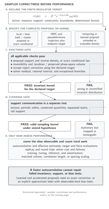
Positive determinant representation identifies the target; solver residuals, rational support, reversible molecular dynamics, and endpoint evaluation determine whether the implemented pseudofermion kernel preserves it. Iteration counts and acceleration claims come afterward. Original schematic, not to scale.

The canonical sampler correctness and performance matrix provides the full determinant, approximation, coverage, bias-test, and cost fields.

Direct two-flavor matrix benchmark

For the convention-card matrix,

$$\det A(u)=(1+u)(4+u), \qquad \frac{d}{du}\log\det A(u)=\frac{1}{1+u}+\frac{1}{4+u}.$$

The effective fermion action is $S_f=-\log\det A$, so its exact derivative is the negative of this trace. At fixed pseudofermion $\phi=(\phi_1,\phi_2)$,

$$S_{\mathrm{pf}}(u)=\frac{|\phi_1|^2}{1+u}+\frac{|\phi_2|^2}{4+u}, \qquad \frac{dS_{\mathrm{pf}}}{du} =-\frac{|\phi_1|^2}{(1+u)^2}-\frac{|\phi_2|^2}{(4+u)^2}.$$

Because $\mathbb E(|\phi_i|^2)=a_i$ under the refreshed conditional, averaging the pseudofermion force gives $-[1/(1+u)+1/(4+u)]$, exactly the determinant force. Between $u=0$ and $u=1$, the determinant ratio is

$$\frac{\det A(1)}{\det A(0)}=\frac{10}{4}=\frac52.$$

This fixture checks Gaussian refresh, inverse application, force sign, determinant ratio, and any factorization without a lattice-fermion implementation. A second stage replaces $A$ by a small explicitly assembled $M^\dagger M$ from the fermion page and compares its direct eigendecomposition, pseudofermion action, force finite difference, and accepted observables.

Adversarial failures

A spectral interval violation. Train or tune a rational approximation on $[10^{-2},10]$ and inject an eigenvalue $10^{-4}$. The nominal maximum error no longer applies. An eigenvalue monitor or direct small-matrix comparison must reject the run.

A recurrence residual mistaken for the true residual. Stop an iterative solve using an internally updated residual that has drifted from $\phi-A\widehat\chi$. Recompute the residual explicitly in higher precision; the action bound and reversal test should expose the defect.

The same loose solve in force and acceptance. If the endpoint Hamiltonian uses an uncontrolled approximation, increasing the Metropolis rejection rate does not guarantee correction to the intended determinant. Tightening the endpoint solve must be an observable stability test, not merely an acceptance study.

A hidden determinant change. Replace $\det M$ by $\det(M^\dagger M)^{1/2}$ without tracking a possible sign or phase. Pseudofermions then sample $|\det M|$, not necessarily the intended theory. No solver tolerance can repair that target mismatch.

Observable-level validation checklist

• State the exact determinant or Pfaffian factor, flavor power, positivity hypothesis, and eigenvalue interval.
• Verify Gaussian refresh and pseudofermion normalization on a diagonal matrix before using an iterative solver.
• Compare direct determinants, log derivatives, forces, and determinant ratios on small matrices; finite-difference the full implemented force.
• Record true solver residuals and iteration counts for force, acceptance, and measurement roles separately; scan each tolerance.
• Measure molecular-dynamics reversibility and correlate outliers with residuals, condition estimates, rational interval excursions, and exceptional branches.
• Inject a sign error, interval violation, stale initial guess, or loose endpoint solve and require an exact or observable test to fail.
• Compare the accepted bosonic observables with a direct determinant calculation on the smallest lattice. Route complex weights to Chapter 8 rather than forcing a positive representation.

Learning outcomes

After completing this page, you should be able to:

• derive pseudofermion representations for positive determinant factors and state when factorization or rational approximation changes only the method rather than the target; and
• bound or exclude solver, rational, and reversibility bias using residuals, spectral intervals, tolerance scans, and an exact small-system determinant fixture.

Exercises

1. Derive the force expectation. For a positive matrix $A(u)$ and $A'=dA/du$, show that the pseudofermion force averaged over refreshed $\phi$ equals the derivative of $-\log\det A$.

Solution

At fixed $u$, $\mathbb E(\phi\phi^\dagger)=A$. Hence $\mathbb E[-\phi^\dagger A^{-1}A'A^{-1}\phi]= -\operatorname{Tr}[A^{-1}A'A^{-1}\mathbb E(\phi\phi^\dagger)]= -\operatorname{Tr}(A^{-1}A')$. Jacobi’s formula gives $d[-\log\det A]/du=-\operatorname{Tr}(A^{-1}A')$.

2. Verify the Hasenbusch identity eigenvalue by eigenvalue. Show positivity of both factors and write their pseudofermion kernels.

Solution

For an eigenvalue $a>0$, $(a+\mu^2)[a/(a+\mu^2)]=a$, and both factors are positive. The first determinant uses action $\phi_1^\dagger(A+\mu^2I)^{-1}\phi_1$. For $B=A(A+\mu^2I)^{-1}$, the second uses $\phi_2^\dagger B^{-1}\phi_2=\phi_2^\dagger(A+\mu^2I)A^{-1}\phi_2$. Multiplying the Gaussian integrals returns $\det A$.

References

• Clark, M. A., and Kennedy, A. D. (2007). “Accelerating staggered-fermion dynamics with the rational hybrid Monte Carlo algorithm.” Physical Review D 75, 011502(R). doi:10.1103/PhysRevD.75.011502; Open PDF.
• Duane, S., Kennedy, A. D., Pendleton, B. J., and Roweth, D. (1987). “Hybrid Monte Carlo.” Physics Letters B 195(2), 216–222. doi:10.1016/0370-2693(87)91197-X.
• Hasenbusch, M. (2001). “Speeding up the Hybrid-Monte-Carlo algorithm for dynamical fermions.” Physics Letters B 519(1–2), 177–182. doi:10.1016/S0370-2693(01)01102-9; Open PDF.