Observables and Dynamics in Truncated Spaces

Observables and real-time evolution require their own effective operators in a truncated space. A Hamiltonian counterterm that stabilizes energies does not automatically stabilize a current, matrix element, spectral weight, or quench. The calculation must dress both states and operators, check exact sum rules, separate Hilbert leakage from finite-volume recurrence, and demonstrate joint improvement as state, operator, cutoff, and time-window approximations are enlarged.

Required background. Basis Construction, Symmetry Sectors, and Matrix Elements supplies normalized states and operator matrices. Renormalizing a Truncated Hamiltonian supplies the omitted-state resolvent and matching scheme. Real-Time Evolution, Scattering, and Observable Extraction supplies the general finite-volume Hamiltonian treatment of time evolution.

Helpful background. Variational Principles and Field-Theory Ansätze supplies projected time evolution and residuals. Retarded, Advanced, and Spectral Correlators supplies causal response and spectral conventions.

Eliminating states also dresses operators

Observable and dynamics contract. Declare the initial state, final state or time-evolution protocol, bare operator normalization, projected and induced operator terms, matching inputs, spectral range or time window, state and operator cutoffs, volume, and every sum-rule or symmetry test. Keep Hamiltonian error, state error, effective-operator error, time-step or Krylov error, leakage, and recurrence as separate entries.

For an eigenvalue $E$ away from the spectrum of $QHQ$, define the wave operator

$$\Omega(E)=P+Q(E-QHQ)^{-1}QHP.$$

If $|\psi_P\rangle=P|\Psi\rangle$, then the exact state is $|\Psi\rangle=\Omega(E)|\psi_P\rangle$. Therefore an exact matrix element is

$$\langle\Psi_f|O|\Psi_i\rangle =\langle\psi_{P,f}| P\Omega^\dagger(E_f)O\Omega(E_i)P |\psi_{P,i}\rangle.$$

The reduced states carry the effective norm $N_{\mathrm{eff}}(E)=P\Omega^\dagger(E)\Omega(E)P$; one may transform to an orthonormal convention or retain this metric explicitly. The effective observable

$$O_{\mathrm{eff}}(E_f,E_i) =P\Omega^\dagger(E_f)O\Omega(E_i)P$$

contains terms in which $O$ acts before, after, or entirely within omitted propagation. The bare projection $POP$ drops them. This is the same projection logic that produces the Feshbach effective Hamiltonian Feshbach 1958, §§ 2–3.

Expanding to first order in the $P$–$Q$ coupling gives, schematically,

$$O_{\mathrm{eff}} =POP +PHQ(E_f-QHQ)^{-1}QOP +POQ(E_i-QHQ)^{-1}QHP+\cdots.$$

Thus operator corrections can begin at a different order from energy corrections and can involve different symmetry channels. Matching only $H_{\mathrm{eff}}$ cannot determine them.

Spectral sums expose missing strength

For a normalized ground state and a Hermitian operator $O$, completeness gives

$$\sum_n|\langle n|O|0\rangle|^2 =\langle0|O^2|0\rangle.$$

Removing the elastic term yields the connected sum rule

$$\sum_{n>0}|\langle n|O|0\rangle|^2 =\langle O^2\rangle_0-\langle O\rangle_0^2.$$

A truncated spectral sum can fail in three distinct ways: high final states are absent, retained eigenstates are distorted, and the operator lacks induced terms. Increasing the number of retained eigenvectors tests only the first. A meaningful check compares the spectral sum with an independently evaluated equal-time expectation using the same matched operator convention, then studies both as the Hilbert and operator bases grow.

For an operator of definite momentum or charge, the sum runs only over the allowed sector. Selection rules therefore supply exact zero tests and make the sum rule more diagnostic than a total norm that mixes sectors.

A two-level quench is an exact leakage benchmark

Take

$$H=\begin{pmatrix}0&g\\g&\Delta\end{pmatrix}, \qquad |\psi(0)\rangle=|0\rangle,$$

and let $P=|0\rangle\langle0|$. Exact evolution gives the probability of occupying the omitted state,

$$P_Q(t) =\frac{4g^2}{\Delta^2+4g^2} \sin^2\!\left(\frac{t}{2}\sqrt{\Delta^2+4g^2}\right).$$

The bare projected Hamiltonian $PHP=0$ predicts $P_Q(t)=0$. Adding only the static second-order energy shift $-g^2/\Delta$ changes the retained phase but still cannot reproduce the transition probability. This exactly checkable example separates a successful energy correction from a failed dynamical observable.

For $|g/\Delta|\ll1$ and times not growing so rapidly that secular errors dominate,

$$P_Q(t)=\frac{4g^2}{\Delta^2} \sin^2\!\left(\frac{\Delta t}{2}\right) +O\!\left(\frac{g^4}{\Delta^4}\right).$$

A correct effective description of this probability must either retain the high state, match an operator sensitive to it, or restrict its claim to low-frequency observables for which the high transition is integrated out.

Finite-volume scalar quenches need three independent windows

For a finite-volume scalar theory, prepare an initial ground state $|\Psi_i\rangle$ of $H(g_i)$ and evolve with $H(g_f)$. In the final eigenbasis,

$$\langle O(t)\rangle =\sum_{m,n}c_m^*c_n e^{i(E_m-E_n)t}O_{mn}, \qquad c_n=\langle n_f|\Psi_i\rangle.$$

This representation separates three truncations: the final-state sum, the initial-state overlap, and the operator matrix. It also exposes phase error: an energy error $\delta E$ produces an order-one phase shift by $t\sim1/|\delta E|$, even when short-time observables look accurate.

The useful time interval is bounded independently by:

• the numerical propagation or Krylov error for the fixed matrix;
• the truncation time over which omitted-state leakage or phase drift stays below tolerance; and
• the finite-volume recurrence time, after which discrete levels produce returns absent from the intended infinite-volume process.

Matrix exponentiation or Krylov convergence controls only the first. The truncated-spectrum literature emphasizes that finite-volume levels and matrix elements together determine dynamical observables James et al. 2018, §§ IV–VII.

The convergence map requires joint state–operator improvement

Inspect the two effective branches in the shared map. A fitted energy plateau can coexist with operator drift, so certification occurs only after both branches pass residual, held-out, cross-basis, and multi-cutoff tests.

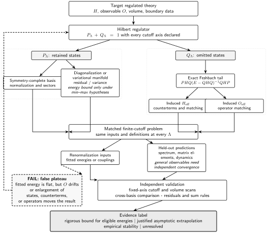
State elimination induces both $H_{\mathrm{eff}}$ and $O_{\mathrm{eff}}$. Spectral sums, leakage, held-out matrix elements, time-window tests, and cross-basis comparisons must converge jointly; only eligible Ritz energies have monotone variational status. The false-plateau branch is schematic and not to scale.

Minimum truncation certification record

Required fields for a truncation result and the test that can falsify each field.

Field	Required declaration	Independent test	Failure signal
Target	Hamiltonian, prior regulator, volume, boundary data, observable	Units and free or exact limit	Changing target across cutoff points
Projectors	PΛ, QΛ, all cutoff axes, limit order	State counts and nestedness	Unidentified omitted states
Basis and sectors	Normalization, Gram matrix, null removal, exact charges	Hermiticity and selection rules	Duplicates or broken constraints
Induced Hamiltonian	Derived operator basis and approximation order	Omitted-state toy model or perturbative coefficient	Drift incompatible with the declared tail
Counterterms	Inputs, running coefficients, and no-double-counting rule	Refit protocol at every cutoff	A fitted datum presented as a prediction
Variational status	Manifold, optimizer, symmetry, bound hypotheses	Residual, variance, and ansatz enlargement	Energy plateau with a large residual
Effective observables	Projected and induced operator terms	Sum rule or matched matrix element	Spectrum stable while the observable drifts
Cutoff sequence	Independent basis, volume, counterterm, time, and state scans	Fixed-axis and cross-term fits	Only one diagonal sequence
Extrapolation	Asymptotic form, fit window, covariance, alternatives	Window and model stability	Exponent chosen from the desired answer
Held-out tests	Unused spectrum, matrix element, dynamics, and second basis	Blind comparison after choices freeze	All tests participated in tuning
Adversarial enlargement	Larger state and operator bases	Repeat the full match and prediction	Former plateau moves beyond its error
Claim	Bound, asymptotic evidence, empirical stability, or unresolved	Error and cost reproduced independently	Precision exceeds the weakest test

Adversarial failure: a stable spectrum and a broken sum rule

Suppose mass and coupling counterterms are tuned so the first two gaps barely change over four cutoffs. The bare projected field operator is then used, and the retained spectral sum reaches a plateau at only $70\%$ of the independently computed connected equal-time variance. The missing $30\%$ may be high-state strength or an induced operator contribution; the stable gaps do not decide between them.

The result cannot support the matrix-element claim. Enlarge the final-state sum at fixed operator, add the derived effective-operator basis at fixed state cutoff, and vary both together. These crossed tests distinguish missing final states from operator matching.

Observable-level validation checklist

• Verify operator Hermiticity in the retained metric and every exact momentum, charge, parity, and Ward selection rule.
• Reproduce the two-level leakage formula and short-time coefficient before a many-state quench.
• Check connected spectral sums against independent equal-time expectation values in each allowed sector.
• Vary Hamiltonian, state, and operator cutoffs independently; repeat the matching protocol at each point.
• Monitor norm, conserved charges, energy where appropriate, Krylov residual, Hilbert leakage estimate, and recurrence indicators.
• Quote a validated time window and show how it changes with cutoff and volume.
• Reserve an unfitted matrix element or response function and reproduce it in a second basis or formulation.

You should now be able to (1) derive the wave-operator expression for a truncated observable and identify the terms omitted by $POP$, and (2) design a scalar-quench validation that separates state, operator, propagation, leakage, and recurrence errors. Convergence, Extrapolation, and Error Certification combines these axes into a quantitative error claim; Benchmark Theories for Truncation Methods supplies exact and interacting stress tests. General real-time extraction returns to Hamiltonian Lattice Field Theory; long-time evolution on tensor-network manifolds continues in Real-Time Tensor-Network Dynamics.

Exercises

Derive the two-level transition probability

Starting from the two-state Hamiltonian above and initial state $|0\rangle$, derive $P_Q(t)$.

Solution

Subtracting $(\Delta/2)I$ leaves $H'=g\sigma_x-(\Delta/2)\sigma_z$ with frequency $\Omega=\sqrt{\Delta^2+4g^2}$. The evolution operator is

$$e^{-iHt}=e^{-i\Delta t/2} \left[\cos\frac{\Omega t}{2}\,I -\frac{2i}{\Omega}\sin\frac{\Omega t}{2}\,H'\right].$$

The transition amplitude is $-2ig\,e^{-i\Delta t/2}\sin(\Omega t/2)/\Omega$. Squaring it gives

$$P_Q(t)=\frac{4g^2}{\Delta^2+4g^2} \sin^2\frac{\Omega t}{2}.$$

Diagnose a partial spectral sum

A retained calculation gives $\sum_{n=1}^{N}|\langle n|O|0\rangle|^2=0.42$, while an independent equal-time calculation gives $\langle O^2\rangle-\langle O\rangle^2=0.50$. What can and cannot be inferred?

Solution

With exact states and operator, completeness would place exactly $0.08$ of spectral weight outside the retained final-state set. In a truncated calculation, however, the $0.08$ can also reflect distorted states or a missing effective-operator term. The discrepancy proves that the present observable calculation is incomplete; it does not uniquely locate the error. One must cross state-count enlargement with operator-basis enlargement and repeat the sum rule at several Hilbert cutoffs.

References

• Feshbach, Herman. “Unified Theory of Nuclear Reactions.” Annals of Physics 5, no. 4 (1958): 357–390. DOI.
• James, Andrew J. A., Robert M. Konik, Philippe Lecheminant, Neil J. Robinson, and Alexei M. Tsvelik. “Non-Perturbative Methodologies for Low-Dimensional Strongly-Correlated Systems: From Non-Abelian Bosonization to Truncated Spectrum Methods.” Reports on Progress in Physics 81, 046002 (2018). DOI.