

Spectral Reconstruction and Ill-Posed Euclidean Inverse Problems
Euclidean data determine only smeared combinations of a continuous spectral density. The Laplace-like kernel suppresses fine spectral structure, its discretization has rapidly decaying singular values, and finitely many noisy time slices leave a large approximate null space. A reconstruction is reliable only when it reports its resolution function, regularization or prior assumptions, mock-data recovery, and negative controls. A stable curve is not evidence of uniqueness.
Required background. Euclidean Correlators and Spectral Information distinguishes measured correlators from inferred spectral quantities.
Helpful background. Retarded, Advanced, and Spectral Correlators defines the Lorentzian spectral object. Branches, Sheets, Analytic Continuation, and Monodromy supplies the analytic-continuation cautions.
In the chapter’s observable-chain table, this page bounds continuous spectral inference at the correlator stage; it does not turn a smeared reconstruction into the discrete bare-matrix-element chain.
The Euclidean integral transform
Section titled “The Euclidean integral transform”At zero temperature, a bosonic Euclidean correlator often has the form
up to normalization conventions and possible subtractions. At temperature , a common kernel is
The spectral density’s sign, oddness, contact terms, and polynomial subtractions depend on the operator and convention. Positivity holds for selected diagonal channels in a positive Hilbert space; it is not universal for off-diagonal, subtracted, gauge-dependent, or fermionic structures.
Inverse-problem conventions. The page uses Euclidean times , the site-wide conventions, and a spectral normalization fixed by the displayed kernel. The frequency interval, quadrature measure, covariance, subtraction terms, positivity constraints, and sum rules are local inputs. Real-time transport or thermal interpretation belongs to Thermal and Nonequilibrium QFT.
After choosing quadrature nodes and weights ,
Typically , so the matrix has an exact null space even before noise. More importantly, its nonzero singular values decay rapidly. A raw singular-value decomposition of diagnoses algebraic rank, but its numerical values depend on the units, frequency binning, and parameter scaling and therefore cannot be compared directly with a “noise level.”
For a quantitative diagnostic, choose a positive spectral-space metric , define unit spectral coordinates , and whiten the data covariance. Then decompose
The whitened noise has unit covariance, and formal inversion still amplifies the th left-singular projection by . Whether that direction is informative depends on its expected signal projection and propagated variance, not on a universal raw- cutoff. The declared metric matters: increasing the frequency grid or rescaling bins can change coordinates but cannot create information.
Resolution functions make the answer inspectable
Section titled “Resolution functions make the answer inspectable”Consider a linear estimator at target frequency ,
Its expectation value is
is the resolution function. The estimator measures a weighted average, not the point value unless the resolution is demonstrably narrow compared with the feature of interest. Its normalization, width, sidelobes, and sign should be reported.
For lattice correlators, a particularly transparent strategy is to choose the target smearing function first and ask which smeared spectral density the data can determine, carrying both statistical uncertainty and approximation error Hansen, Lupo, and Tantalo 2019, §§2–4. This reverses the misleading order in which a finely binned pointwise spectrum is drawn first and its actual resolution is discussed afterward.
Backus–Gilbert methods choose to minimize a resolution-width functional subject to normalization, with covariance regularization controlling variance Backus and Gilbert 1968. Tikhonov methods instead solve
The operator , reference , and parameter encode a smoothness or size assumption. The resolution matrix is
Rows of show which combinations of the discretized spectrum are actually returned. Quoting without hides the estimator’s effective smoothing.
The reference model contributes to the expectation as well. When the displayed normal matrix is invertible,
Thus the rows of resolve deviations from ; unresolved directions revert to the reference model. Varying while holding one favorable fixed does not test this bias. With constraints or a generalized inverse the estimator need not remain linear, but the same question—what part of the answer comes from the reference or prior—still has to be answered.
Bayesian reconstruction states additional information probabilistically
Section titled “Bayesian reconstruction states additional information probabilistically”A Bayesian analysis defines
The prior may impose positivity, smoothness, sparsity, asymptotic behavior, or a default model. These can be scientifically justified, but they remain assumptions beyond the likelihood. Posterior concentration does not imply data identification if the posterior largely reproduces the prior in poorly constrained singular directions.
Report at least:
- prior predictive correlators and whether they cover the observed scale;
- posterior-to-prior change in the derived feature;
- sensitivity to scientifically plausible hyperpriors or default models;
- resolution or influence diagnostics in data space; and
- coverage on mock spectra not generated from the inference prior.
Maximum entropy and related Bayesian methods are described systematically by Jarrell and Gubernatis 1996, §§3–6. Their value does not remove the need to distinguish data-supported averages from prior-supported shape.
A broad-peak mock example
Section titled “A broad-peak mock example”Use dimensionless units and choose the positive synthetic spectrum
with
Discretize with , use for , and generate by midpoint quadrature. A reproducible correlated-noise model is
Freeze the random seed or publish the generated data vector. The validation question is not whether the reconstructed curve resembles the input. It is whether derived features—integrated weight in a declared window, centroid after convolution with the resolution function, or the existence of a peak broader than the resolution—achieve calibrated coverage. Report the chosen estimator weights, resolution width and sidelobes, the recovered smeared quantity, its propagated uncertainty, and coverage across independently seeded replicas.
Construct two negative controls:
- replace the peak by a smooth shoulder whose correlator difference obeys ;
- add a high-frequency oscillatory function chosen so lies below the noise level while remains allowed.
If the method claims to distinguish either pair, it is using regularization or prior information. That may be acceptable, but the claim must be conditional on it.
The QFT.org 2026 Chapter 2 benchmark, validated snapshot gives a minimal exact version of the second control: two Euclidean times and three frequency bins produce a nonzero null vector by construction. Two distinct positive spectra separated along that vector return the same correlator to floating-point precision. The example is intentionally small enough that every matrix entry and positivity condition can be inspected.
It also freezes a noiseless quadrature check with
and a normalized Gaussian resolution centered at with standard deviation . Midpoint grids with and bins agree in the smeared value to the declared relative tolerance; the finer grid returns and reconstructs the resolution width as . This verifies quadrature and convolution bookkeeping. Coverage under the correlated-noise protocol above remains a separate ensemble test rather than something a noiseless fixture can establish.
Sum rules and positivity help but do not cure nonuniqueness
Section titled “Sum rules and positivity help but do not cure nonuniqueness”An exact or independently renormalized sum rule
adds one linear constraint. Positivity replaces a linear space by a convex cone. Both can substantially bound integrated quantities, yet a finite collection of constraints still admits many spectra. Test the sum rule on the same renormalization and subtraction convention; otherwise its apparent violation may be a scheme mismatch.
Moments obtained from derivatives near are often contaminated by contact terms and ultraviolet divergences. Treating them as exact constraints without matched subtractions can worsen, rather than improve, the inverse problem.
Adversarial failure cases
Section titled “Adversarial failure cases”Frequency bins called resolution. A grid spacing is chosen by the analyst. Resolution is determined by the kernel, time coverage, covariance, and regularization.
A stable peak under one parameter scan. Several regularization values can return nearly identical curves because they share the same prior family. Mock alternatives test identifiability more directly.
Positivity imposed on an ineligible channel. Verify the operator and spectral convention before constraining .
Covariance eigenmodes discarded silently. Regularizing data covariance and regularizing the inverse spectrum are distinct operations; report both.
Euclidean fit quality used as real-time validation. Many spectra produce indistinguishable Euclidean correlators. A good forward fit is necessary, not sufficient.
The map below separates the resolution-limited continuous-spectrum branch from finite-volume state isolation. Follow the lower branch: regularization and a resolution function constrain what the Euclidean data identify, while renormalization and continuum inference remain subsequent operations.
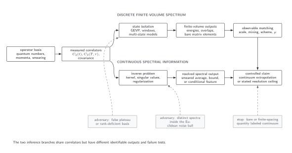
Two inference problems share the same regulated correlators. Discrete energies and overlaps, together with validated connected and disconnected three-point estimators, support bare matrix elements that require matching and continuum control before becoming physical results. Continuous reconstruction identifies only smeared averages, bounds, or conditional features at the demonstrated resolution; without separate matching and continuum analysis it ends at a methodological ceiling. Dashed boxes mark failure tests. The diagram is schematic and not to scale.
Observable-level validation checklist
Section titled “Observable-level validation checklist”Before reporting spectral information, require:
- the exact kernel, normalization, subtractions, frequency domain, and covariance;
- the data-whitening convention, spectral metric, singular projections, and propagated variances;
- resolution functions or an equivalent influence matrix;
- regularization and prior assumptions varied over scientifically meaningful alternatives;
- forward residuals evaluated with the full covariance;
- mock recovery with features both broader and narrower than the attainable resolution;
- negative controls drawn from the approximate null space;
- positivity and sum rules justified for the precise channel; and
- the final claim stated as a resolved average, bound, or conditional feature rather than an unqualified pointwise spectrum.
Exercises
Section titled “Exercises”1. Null-space nonuniqueness. Let be an matrix with . Show that a noiseless solution is nonunique whenever an allowed nonzero lies in .
Solution
If and , then . Positivity or other constraints may exclude some , but unless they remove the entire admissible null direction the data alone cannot choose between the spectra.
2. Resolution bias. Suppose the estimator has a translation-invariant normalized Gaussian resolution of standard deviation , while the true spectrum contains a Gaussian peak of standard deviation far enough from the boundary that half-line truncation is negligible. What width is observed?
Solution
With both widths defined as standard deviations and the stated translation-invariant, effectively full-line approximation, convolution of Gaussians adds variances, so the observed width is . Near the boundary, or for a frequency-dependent or non-Gaussian resolution, the returned shape need not be Gaussian and this formula does not apply. A measured width comparable with cannot establish a narrow intrinsic peak without deconvolution assumptions that the Euclidean data may not support.
What you can now do
Section titled “What you can now do”You should now be able to compute a resolution function, identify approximate null directions, and separate likelihood-supported spectral averages from regularization- or prior-supported structure. Real-time transport and thermal interpretation continue in Thermal and Nonequilibrium QFT.
References
Section titled “References”- Backus, George, and Freeman Gilbert. “The Resolving Power of Gross Earth Data.” Geophysical Journal of the Royal Astronomical Society 16, no. 2 (1968): 169–205. doi:10.1111/j.1365-246X.1968.tb00216.x.
- Hansen, Martin, Alessandro Lupo, and Nazario Tantalo. “On the Extraction of Spectral Densities from Lattice Correlators.” Physical Review D 99, no. 9 (2019): 094508. doi:10.1103/PhysRevD.99.094508.
- Jarrell, Mark, and J. E. Gubernatis. “Bayesian Inference and the Analytic Continuation of Imaginary-Time Quantum Monte Carlo Data.” Physics Reports 269, no. 3 (1996): 133–195. doi:10.1016/0370-1573(95)00074-7.
- QFT.org. “Lattice Observables and Continuum Inference Benchmark.” JavaScript source, validated 25 August 2026. SHA-256
d76924d8c724cb7c9307fb38265336495fa3ff1a98103b3fa4fa734262647c2a. Reproducibility record.
Further reading
Section titled “Further reading”- Meyer, Harvey B. “Transport Properties of the Quark–Gluon Plasma: A Lattice QCD Perspective.” European Physical Journal A 47 (2011): 86. doi:10.1140/epja/i2011-11086-3.