Massless Fields, Long-Range Forces, and Finite-Volume QED

A massless field removes the contour gap that makes ordinary wrapping effects exponential. Finite-volume corrections then fall as powers of $1/L$, depend on box shape and zero-mode treatment, and may reflect a modified finite-volume theory rather than a passive approximation to infinite-volume QED. On a periodic torus, Gauss’s law also forbids a net charge unless the zero mode, boundary conditions, or charge constraint is changed. A charged observable is therefore defined only after a finite-volume prescription and its matched infinite-volume target have been named.

Required background. Finite Volume as a Controlled Deformation supplies the branch and limit-order tests. Massless Scalars, Zero Modes, and Infrared Limits supplies the nonuniform massless limit.

Helpful background. Charges, Screening, and Long-Range Forces supplies Gauss-law and screening physics. Dressed States and Infrared-Finite Scattering explains why exclusive charged-particle amplitudes require a separate infinite-volume infrared treatment.

Gauss’s law and the missing photon zero mode

Integrating Gauss’s law over a compact periodic spatial volume gives

$$Q_{\rm tot} =\int_{L^3}\!\mathrm d^3x\,\rho =\int_{L^3}\!\mathrm d^3x\,\boldsymbol\nabla\cdot\mathbf E =\oint_{\partial L^3}\!\mathbf E\cdot\mathrm d\mathbf S =0,$$

because opposite faces cancel. Naive periodic Maxwell theory therefore has no gauge-invariant state of nonzero total charge. Removing a photon zero mode or changing the boundary data changes this conclusion by changing the theory.

Long-range finite-volume prescription. The quantitative benchmark uses a named photon zero-mode prescription and a specified order of limits; changing either defines a different finite-volume theory and power counting.

For the quantitative benchmark, the detailed choices are:

Field	Choice used on this page
Prescription	$\mathrm{QED}_{\mathrm L}$: remove every photon mode with spatial momentum $\mathbf k=\mathbf0$, for every Euclidean frequency $k_0$
Geometry	Periodic cubic space of side $L$; take $T\to\infty$ before quoting the displayed mass shift
Coupling	$\alpha=e^2/(4\pi)$ and charge $Qe$; the benchmark uses $\alpha=1/137$ and $Q=1$
Observable	Pole mass of a stable point particle, compared at fixed renormalized infinite-volume mass $M$
Locality statement	Spatial zero-mode removal is nonlocal in space; effective descriptions must respect that prescription rather than assume a local finite-volume EFT
Target	Infinite-volume QED after the prescribed $L\to\infty$ limit; no claim about an exclusive charged-particle S-matrix element is inferred

The spatial zero-mode removal is

$$A_\mu(k_0,\mathbf0)=0 \quad\text{for every }k_0.$$

It preserves spatial cubic symmetry and a useful transfer interpretation, but it is nonlocal in space. Davoudi and collaborators analyze precisely these properties and the consequences for effective descriptions (Davoudi et al. 2019, §§ II–IV); the finite-volume-QED prescription and hadron-mass scaling were introduced in this form by Hayakawa and Uno 2008, §§ 2–4.

Other prescriptions are not interchangeable labels:

Prescription class	Modification	Consequential check
$\mathrm{QED}_{\mathrm L}$	Remove all $\mathbf k=0$ photon modes	Verify the known $1/L$ and $1/L^2$ point-particle terms and state spatial nonlocality
$\mathrm{QED}_{\mathrm{TL}}$	Remove only the four-momentum zero mode	Keep $T/L$ explicit; the $T\to\infty$ limit at fixed $L$ is not automatically benign
Charge-conjugation or other nonperiodic boundaries	Change field identifications so flux need not cancel face by face	Verify the allowed charge sectors and the altered momentum grid
Massive-photon regulator	Add a photon mass $m_\gamma$ and later remove it	Control both $m_\gamma L$ and the noncommuting $m_\gamma\to0$, $L\to\infty$ limits

The prescription must also be used consistently in sea and valence sectors, operator renormalization, effective theory, and finite-volume correction. A hybrid calculation can have a formally correct coefficient for the wrong theory.

Power counting from the sum–integral difference

For a massless propagator, the finite-volume residue of a loop contains

$$\left[ \frac{1}{L^3}\sum_{\mathbf k}^{\prime} -\int\frac{\mathrm d^3k}{(2\pi)^3} \right]\frac{1}{\mathbf k^2},$$

where the prime implements the chosen zero-mode rule. Rescaling $\mathbf k=\mathbf q/L$ shows that the expression has dimension $L^{-1}$. There is no mass scale available to generate $e^{-mL}$; the leading charged self-energy must be proportional to $\alpha Q^2/L$ times a shape coefficient. Higher terms introduce $1/(ML)$, structure scales, and prescription-dependent coefficients.

In the stated $\mathrm{QED}_{\mathrm L}$ benchmark,

$$\Delta M(L) =M(L)-M(\infty) =\frac{\alpha Q^2c_1}{2L} +O\!\left(\frac{\alpha}{ML^2}\right), \qquad c_1=-2.837297479\ldots.$$

For $Q=1$ and $\alpha=1/137$, the dimensionless leading shifts are

$ML$	$\Delta M/M$ from the displayed term
4	$-2.59\times10^{-3}$
6	$-1.73\times10^{-3}$
8	$-1.29\times10^{-3}$

The product $L\Delta M$ is constant at this order, so these three values form an exact scaling fixture for the declared prescription. The coefficient and its extensions for composite hadrons are derived in Davoudi and Savage 2014, §§ II–III. This row is not a full-QED prediction: structure-dependent terms, strong finite-volume effects, discretization, and higher orders remain.

Neutrality does not restore exponential behavior universally. A neutral composite particle can couple through multipole moments or polarizabilities, so its leading electromagnetic correction may begin at a higher power of $1/L$. Conversely, screening or a photon mass can reinstate an exponential scale, but only after the screening length or $m_\gamma^{-1}$ is included in the hierarchy.

Prescription comparison is a matching problem

To compare two finite-volume QED prescriptions:

1. specify their allowed field modes, gauge transformations, charge sectors, symmetries, locality properties, and temporal limit;
2. compute the same renormalized, infrared-safe target observable in each;
3. subtract each prescription’s own analytic power corrections through a common order;
4. take its prescribed limits; and
5. compare the common infinite-volume observable, not the raw finite-$L$ masses.

The finite-$L$ difference between prescriptions is generally expected and is not itself a physical disagreement. Universality concerns the matched limit. Current rankings, implementation performance, and evolving comparisons belong to the Lattice and Hamiltonian Field Theory Research area.

The branch map below makes that boundary explicit. The durable content is a fully specified prescription plus exact tests; coupled, current, and three-body branches require their own dated status rather than inheriting validation from the same upstream spectrum.

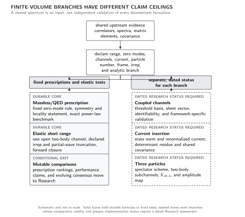
Finite-volume branches have different claim ceilings. A fixed massless-field prescription and an exact power-law test are durable; mutable prescription comparisons may move to Research. Coupled-channel, current-insertion, and three-particle claims require separate dated status and validation. The map is schematic and not to scale.

Adversarial tests and stop rules

False exponential. Fitting $M(L)=M_\infty+Ae^{-mL}$ to three modest volumes can approximate a $1/L$ drift. Reject the model by examining $L\Delta M$, by adding a larger volume, and by checking the analytic coefficient under the declared zero-mode rule.

Unmatched prescriptions. Agreement after subtracting the $\mathrm{QED}_{\mathrm L}$ coefficient from data generated with a different zero-mode rule is accidental. Stop until the data-generating action and correction formula use the same modes.

Wrong observable. A finite-volume charged two-point pole mass may be well-defined under a prescription, but it does not by itself define an infrared-finite exclusive scattering amplitude. Stop at the mass unless the infinite-volume inclusive or dressed observable has been separately specified.

The spectrum-to-amplitude map shows why a massless prescription cannot be silently inserted into the short-range branch. Follow the dashed path from the finite-volume level: the zero-mode prescription and its power-law corrections must be fixed before any infinite-volume interpretation.

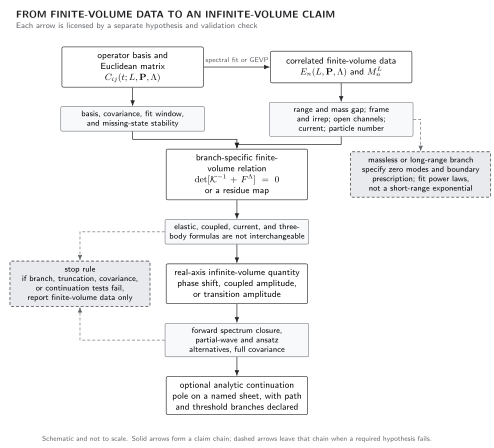
Finite-volume information reaches an infinite-volume claim only through a branch-specific map. Solid arrows show the controlled chain; dashed arrows show the long-range alternative and the stop rule. The image is schematic, not to scale, and the displayed determinant is structural: its channel, irrep, partial-wave, normalization, and sign conventions must be fixed locally.

Observable-level validation

Before reporting a long-range finite-volume result, verify that:

• the photon or massless-field mode set, boundary conditions, gauge fixing, charge constraint, box shape, and $T/L$ limit are reproducible;
• Ward identities and the allowed charge sectors hold for that prescription;
• an exact free or point-particle sum–integral benchmark reproduces the sign and coefficient of the leading power;
• fits separate strong exponential corrections from electromagnetic powers and include their covariance;
• the first omitted structure-dependent and higher-order terms are varied; and
• only the matched infinite-volume, infrared-safe observable is compared across prescriptions.

What you can now do

You can now (1) write a complete finite-volume massless-field prescription, including zero modes, symmetries, locality, temporal limit, and target observable, and (2) reproduce the $1/L$ scaling fixture above and distinguish its universal charge dependence from prescription- and structure-dependent higher coefficients.

Return to Finite Volume as a Controlled Deformation to compare branch hypotheses. Continuum QED and its physical applications belong to Gauge Theories and the Standard Model.

Exercises

1. Gauss-law obstruction. Why can a uniform compensating background allow a nonzero particle charge without contradicting the integrated equation above?

Solution

The background contributes charge $-Q$, so the total charge on the torus remains zero even though the localized particle carries $Q$. The construction changes the finite-volume theory and its energy by background- and shape-dependent terms; it does not evade Gauss’s law.

2. Scaling discriminator. If the leading correction is $B/L$, compute $\Delta M(2L)/\Delta M(L)$. Compare with a leading $Ae^{-mL}$ correction.

Solution

The power correction gives $1/2$. The exponential gives $e^{-mL}$, which varies with the original $L$ and becomes much smaller when $mL\gg1$. Measuring several widely separated volumes distinguishes them more reliably than fitting a narrow range.

References

• Davoudi, Zohreh, James Harrison, Andreas Jüttner, Antonin Portelli, and Martin J. Savage. “Theoretical Aspects of Quantum Electrodynamics in a Finite Volume with Periodic Boundary Conditions.” Physical Review D 99 (2019): 034510. DOI. Open PDF.
• Davoudi, Zohreh, and Martin J. Savage. “Finite-Volume Electromagnetic Corrections to the Masses of Mesons, Baryons and Nuclei.” Physical Review D 90 (2014): 054503. DOI. Open PDF.
• Hayakawa, Masashi, and Shunpei Uno. “QED in Finite Volume and Finite Size Scaling Effect on Electromagnetic Properties of Hadrons.” Progress of Theoretical Physics 120 (2008): 413–441. DOI.