Hybrid Monte Carlo and Symplectic Molecular Dynamics

Hybrid Monte Carlo (HMC) is exact at finite regulator when a momentum refresh augments the target, a deterministic molecular-dynamics proposal is reversible and volume preserving, and a Metropolis test uses the actual Hamiltonian change. Symplectic integration makes large, coherent field moves with small energy error; it does not by itself preserve the Boltzmann distribution. The acceptance correction removes step-size bias only if the implemented map satisfies the reversibility and Jacobian hypotheses used in the proof.

Required background. Local, cluster, and global update families supplies transition-kernel invariance and Metropolis correction. Hamiltonian evolution, initial data, and phase space supplies canonical flow and Liouville volume.

Helpful background. Constraints, Dirac brackets, and reduction supplies the geometric language needed when fields live on constrained manifolds or gauge groups.

Extended target and fictitious Hamiltonian

Let $q\in\mathbb R^N$ denote all regulated field variables and let the desired density be $\pi(q)\propto e^{-S(q)}$. Introduce momenta $p$ with a symmetric positive-definite mass matrix $M$ and extended density

$$\widetilde\pi(q,p)\propto e^{-H(q,p)}, \qquad H(q,p)=S(q)+\frac12p^{\mathsf T}M^{-1}p.$$

Integrating the Gaussian momenta returns a constant times $e^{-S(q)}$, so discarding $p$ after each trajectory leaves the desired field target. The fictitious equations

$$\dot q=M^{-1}p, \qquad \dot p=-\nabla S(q)$$

are an algorithmic device. Their trajectory time is not the physical real time of a Hamiltonian lattice field theory.

Local regulator and convention card. The derivation uses unconstrained real fields, canonical volume $dq\,dp$, a position-independent mass matrix, and momentum reversal $R(q,p)=(q,-p)$. One leapfrog step has size $\epsilon$; $L$ steps give trajectory length $\tau=L\epsilon$. The interacting benchmark is a periodic four-site scalar with $S(q)=\sum_{i=1}^4[\frac12(q_{i+1}-q_i)^2+\frac{m^2}{2}q_i^2+\frac{\lambda}{4!}q_i^4]$, $q_5=q_1$, $m^2>0$, and $\lambda\ge0$. The analytic unit test sets $N=1$, $S(q)=q^2/2$, and $M=1$.

An HMC update consists of four logically separate operations:

1. Draw $p\sim N(0,M)$ while keeping $q$ fixed.
2. Apply a deterministic numerical map $\Phi_{\epsilon,L}$ approximating Hamiltonian flow.
3. Include momentum reversal in the proposal, $T=R\circ\Phi_{\epsilon,L}$.
4. Accept $z'=Tz$, $z=(q,p)$, with $\alpha(z,z')=\min(1,e^{-[H(z')-H(z)]})$; on rejection retain $q$.

Partial refreshment and persistent momenta are possible, but then their transition and reverse probability must be included explicitly. The basic proof below applies to the full Gaussian refresh; Neal 2011, §§3–5 develops the broader HMC construction and tuning geometry.

Leapfrog, reversibility, and unit Jacobian

For a separable Hamiltonian, one leapfrog step is

$$\begin{aligned} p_{n+1/2}&=p_n-\frac{\epsilon}{2}\nabla S(q_n),\\ q_{n+1}&=q_n+\epsilon M^{-1}p_{n+1/2},\\ p_{n+1}&=p_{n+1/2}-\frac{\epsilon}{2}\nabla S(q_{n+1}). \end{aligned}$$

Each kick is a shear $(q,p)\mapsto(q,p-f(q))$ and each drift is a shear $(q,p)\mapsto(q+g(p),p)$. Their triangular Jacobians have determinant one, so their composition preserves phase-space volume. The symmetric kick–drift–kick order also gives

$$R\Phi_{\epsilon,L}R=\Phi_{\epsilon,L}^{-1}.$$

Consequently $T=R\Phi_{\epsilon,L}$ is an involution, $T^2=1$, and $|\det DT|=1$. These two identities—not the informal resemblance to continuous mechanics—supply the proposal symmetry.

For an invertible deterministic map with unit Jacobian, accepted probability current between $z$ and $z'=Tz$ is

$$e^{-H(z)}\min\{1,e^{-H(z')+H(z)}\} =\min\{e^{-H(z)},e^{-H(z')}\},$$

which is symmetric. Rejection supplies the diagonal term, and the momentum refresh preserves its Gaussian conditional. This derives the HMC ratio used by Duane et al. 1987, pp. 216–222.

If a deterministic proposal has Jacobian $J(z)=|\det DT(z)|\ne1$, the general transformed-density ratio contains $J(z)$. Using the standard $e^{-\Delta H}$ correction while silently omitting a nonunit Jacobian is biased. Likewise, an adaptive stopping rule based on the forward trajectory can make $T$ non-involutive even when every individual step is symplectic.

The HMC branch in the figure below makes this dependence explicit. Inspect the exactness gate before the invariant-kernel box: reversibility, phase-space volume, endpoint acceptance, and numerical target evaluation are separate conditions.

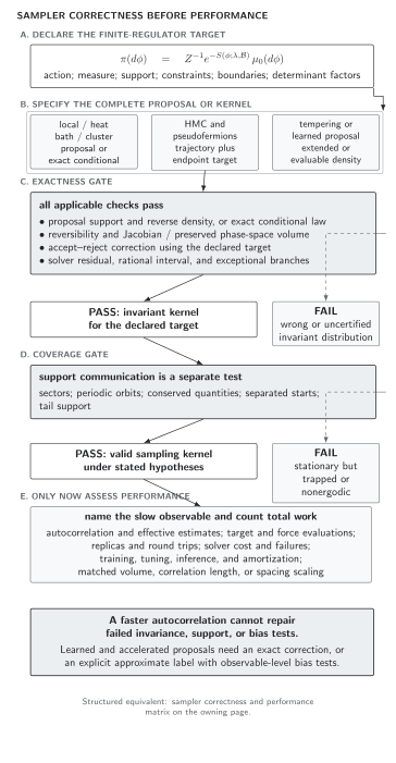
For HMC, symplectic integration supplies a unit-Jacobian proposal and symmetric splitting supplies reversibility; the endpoint Metropolis test then corrects energy error. Coverage and trajectory cost are evaluated only for the resulting invariant kernel. Original schematic, not to scale.

The canonical sampler correctness and performance matrix lists the HMC-specific diagnostics beside those of the other kernels.

An analytic one-step fixture

For $H=(q^2+p^2)/2$, one leapfrog step is the linear map

$$\begin{pmatrix}q'\\p'\end{pmatrix} = \begin{pmatrix} 1-\epsilon^2/2 & \epsilon\\ -\epsilon(1-\epsilon^2/4) & 1-\epsilon^2/2 \end{pmatrix} \begin{pmatrix}q\\p\end{pmatrix}.$$

The determinant is exactly one. At $(q,p)=(0,1)$ and $\epsilon=1/2$, the integrator gives $(q',p')=(1/2,7/8)$. Hence

$$H_0=\frac12=\frac{64}{128}, \qquad H_1=\frac12\left(\frac14+\frac{49}{64}\right)=\frac{65}{128}, \qquad \Delta H=\frac{1}{128},$$

and the exact acceptance probability for this proposal is $e^{-1/128}$. With the final momentum flip included, applying the same proposal twice returns $(0,1)$ exactly in rational arithmetic. This single fixture independently tests the force sign, both half-kicks, update order, determinant, reversibility, Hamiltonian evaluation, and acceptance exponent.

For a smooth stable trajectory, leapfrog has global state error $O(\epsilon^2)$ over fixed $\tau$ and a bounded oscillatory energy error governed by a nearby shadow Hamiltonian; the accepted chain nevertheless targets the original $H$, not the shadow Hamiltonian. Symplectic and reversible integration underlies this behavior Hairer, Lubich, and Wanner 2006, Chs. VI–IX.

Interacting scalar application

Use the four-site $\phi^4$ action in the convention card and differentiate the action independently of the molecular-dynamics routine:

$$\frac{\partial S}{\partial q_i} =2q_i-q_{i-1}-q_{i+1}+m^2q_i+\frac{\lambda}{6}q_i^3.$$

One accepted trajectory is “exact” in the Markov-chain sense: finite $\epsilon$ changes proposal efficiency, while the Metropolis step removes its equilibrium step-size error. A trustworthy first study performs the following hierarchy.

• Compare the analytic gradient with centered finite differences at generic, large, and symmetry-related fields.
• Measure $\|T(Tz)-z\|$ after a forward trajectory, momentum reversal, and the corresponding return; tighten arithmetic or solver tolerances and verify the expected plateau.
• Check that the distribution satisfies $\langle e^{-\Delta H}\rangle=1$ within uncertainty when trajectories start from equilibrium and the map is reversible and volume preserving. This is a diagnostic, not a replacement for observable tests.
• For $V=1$ or $2$, compute $\langle q^2\rangle$ and $\langle q^4\rangle$ by independent high-precision quadrature. For $V=4$, compare with an independently implemented local Metropolis or heat-bath-compatible kernel under matched action and boundaries.
• Repeat over $\epsilon$ at fixed $\tau$. Reversibility residuals and accepted observables should remain stable; $\Delta H$ and acceptance should change. A drift in observables with $\epsilon$ signals a failed correction or numerical irreversibility.

Step size, trajectory length, mass preconditioning, and multiple time scales determine efficiency. Current implementation and hardware performance belong in dated Research benchmarks, not in a durable correctness claim.

Fields on groups and constrained spaces

For a compact gauge link $U$, momenta lie in the Lie algebra and the drift is an exponential update such as $U\mapsto e^{\epsilon P}U$. The target reference measure is Haar measure, not unconstrained Lebesgue measure. A valid integrator must preserve the appropriate cotangent-bundle volume and reverse under $P\mapsto-P$. Projecting an unconstrained matrix back onto the group after a drift is generally not the same map and can introduce an untracked Jacobian or a nonreversible branch. Holonomic constraints likewise require a constraint-preserving, reversible proposal and a measure derived for the reduced space; the general geometry is handled in the linked constraints chapter.

Adversarial failures

Acceptance without a Jacobian. Insert $q\mapsto(1+\delta)q$ into an otherwise valid trajectory and continue to accept with $e^{-\Delta H}$. The map has determinant $(1+\delta)^N$. Energy-based acceptance alone cannot correct the omitted volume factor.

A nearly reversible adaptive trajectory. Stop when $|\Delta H|$ first crosses a threshold. The reverse trajectory generally stops at a different step. High average acceptance may coexist with a measurable $T^2-1$ residual and a biased target.

A force and energy mismatch. Generate forces from one boundary condition or action coefficient but evaluate acceptance with another. If the resulting deterministic map remains reversible and volume preserving, the exact endpoint Hamiltonian can still correct it in principle, but efficiency collapses; history-dependent approximations or inconsistent branching can also destroy reversibility. The implemented map—not an ideal formula—must be tested.

Rounding hidden by a loose tolerance. Report only the median reversal error. Rare large residuals near stiff regions can control bias. Plot the residual against $\Delta H$, solver iterations, and field norm, and compare observables while tightening tolerances.

Observable-level validation checklist

• Declare the extended target, momentum law, mass matrix, integrator order, step size, number of steps, trajectory randomization, and boundary conditions.
• Verify each elementary map’s Jacobian or symplectic property and the implemented identity $R\Phi R=\Phi^{-1}$, including exceptional branches.
• Reproduce the rational Gaussian one-step fixture and finite-difference the interacting scalar force.
• Measure signed and absolute $\Delta H$, $\langle e^{-\Delta H}\rangle$, acceptance, and forward–reverse residuals; do not infer exactness from any one diagnostic.
• Compare even scalar moments with quadrature or an independent kernel and repeat across step sizes and separated starts.
• Inject a nonunit scaling, a missing half-kick, or an asymmetric stopping rule and require the Jacobian, reversibility, or observable check to fail.

Learning outcomes

After completing this page, you should be able to:

• derive the HMC acceptance ratio from an involutive, volume-preserving molecular-dynamics proposal; and
• test reversibility, Jacobian preservation, energy error, acceptance, and observable agreement independently on analytic and interacting scalar fixtures.

Exercises

1. Verify the Gaussian map. Derive the displayed leapfrog matrix and prove that its determinant is one for every $\epsilon$.

Solution

The first kick gives $p_{1/2}=p-\epsilon q/2$. The drift gives $q'=(1-\epsilon^2/2)q+\epsilon p$. Substitution into the second kick yields $p'=(1-\epsilon^2/2)p-\epsilon(1-\epsilon^2/4)q$. The determinant is $(1-\epsilon^2/2)^2+\epsilon^2(1-\epsilon^2/4)=1$.

2. Find the missing correction. Let an involutive differentiable proposal $T$ have nonunit Jacobian. Derive its deterministic Metropolis ratio.

Solution

Conservation of probability under $z'=Tz$ introduces the change-of-variables factor $|\det DT(z)|$. Detailed balance is obtained with $\alpha(z,Tz)=\min\{1,e^{-H(Tz)+H(z)}|\det DT(z)|\}$. For an involution, $|\det DT(Tz)|=|\det DT(z)|^{-1}$, so the reverse ratio is reciprocal. Standard HMC is the special case with unit determinant.

References

• Duane, S., Kennedy, A. D., Pendleton, B. J., and Roweth, D. (1987). “Hybrid Monte Carlo.” Physics Letters B 195(2), 216–222. doi:10.1016/0370-2693(87)91197-X.
• Hairer, E., Lubich, C., and Wanner, G. (2006). Geometric Numerical Integration: Structure-Preserving Algorithms for Ordinary Differential Equations, 2nd ed. Springer. doi:10.1007/3-540-30666-8.
• Neal, R. M. (2011). “MCMC using Hamiltonian dynamics.” In S. Brooks, A. Gelman, G. L. Jones, and X.-L. Meng (eds.), Handbook of Markov Chain Monte Carlo, pp. 113–162. Chapman & Hall/CRC. arXiv:1206.1901.