Equilibration, Stationarity, and Chain Diagnostics

Transition-kernel correctness describes an infinite stationary process; a stored ensemble is one finite realization that may retain its initial condition, drift between regions, or miss a slow sector. Equilibration and stationarity therefore require evidence from multiple starts, slow observables, distributional comparisons, and independent streams. A thermalization cut chosen because it makes the target result look stable is not a valid diagnostic.

Required background. Autocorrelation times define slow realized modes, while algorithm validation and ensemble provenance establish the generation recipe and immutable ensemble identity.

Helpful background. Covariance and resampling preserve stream and block structure after the cut.

Initial-condition bias

Local realized-chain convention and regime. Each stream retains its initial state, update unit, rejected configurations, burn-in candidates, and sector history; stationarity is not assumed from kernel correctness. Cut rules and comparison tolerances are fixed without access to the unblinded target, and every mean, split, or distributional comparison uses autocorrelation-aware uncertainty. These diagnostics assess the finite histories in hand and do not prove transition-kernel invariance.

For a reversible Markov kernel with equilibrium distribution $\pi$, an observable expectation from initial distribution $\nu_0$ has a spectral form

$$\mathbb E_{\nu_0}X_t-\mathbb E_\pi X =\sum_{j\ge1}c_j\lambda_j^t,$$

where $\lvert\lambda_j\rvert<1$ for mixing modes. A start with small overlap $c_j$ can hide a very slow $\lambda_j$ in one observable. Use deliberately overdispersed starts, including ordered/disordered or distinct topological sectors where relevant, and compare their trajectories in several observables.

A cut $t_{\mathrm{burn}}$ should be fixed by a rule—such as agreement of late windows across starts within a declared tolerance—before examining the blinded target. Discarded updates remain part of provenance. The limits of finite-run convergence diagnosis are emphasized in Geyer 1992, pp. 473–483.

Trace, split, and distributional checks

No single diagnostic proves stationarity. Combine:

• trace plots and running means of slow and target observables;
• early/late window comparisons with autocorrelation-aware errors;
• split-chain means and variances across independent streams;
• histograms or empirical distributions, not only means;
• change-point or drift tests with multiple-testing implications stated;
• sector-transition counts and replica agreement.

The common $\widehat R$ idea compares between-chain and within-chain variation, but short chains can agree while all remain trapped in the same region, and overdispersed starts are necessary for interpretation Gelman and Rubin 1992, pp. 457–472. Rank-normalized, folded, and localized refinements improve sensitivity but remain diagnostics rather than proofs Vehtari et al. 2021, pp. 667–718. Effective sample size computed before stationarity is established has no equilibrium meaning.

Adversarial failures: initialization transients and late drift

An initialization transient

$$X_t=3e^{-t/40}+\epsilon_t$$

can look stationary in a short late window yet bias an early average. Multiple starts with opposite or different offsets and a cut scan reveal it.

A late drift

$$X_t=\epsilon_t+0.75\,\mathbf1_{t\ge384}$$

passes any diagnostic restricted to the first half. Split comparisons and running distributions flag the shift. These adversaries should be rejected, not folded into a stationary coverage ensemble.

Independent reproduction

There are two useful levels:

1. independent analysis: a different implementation or analyst starts from the same immutable configurations;
2. independent regeneration: a distinct validated run recreates the estimand from the action and parameter specification.

The first detects analysis and software errors; the second additionally probes ensemble generation and equilibration. Independence is reduced if both use the same cached derived data, random-number stream, code path, or fit-selection script.

Record action and parameter hashes, lattice geometry, code revision, compiler/runtime, random-number generator and seeds, stream ancestry, update counts, acceptance and solver histories, configuration checksums, cut rule, measurement code, and analysis inputs. Reader-facing results need not display internal workflow metadata, but reproducibility records must retain it.

The graph places stationarity before any resampling or fit.

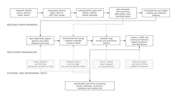
Stationarity is a gate on the realized history, not a property conferred by later blocking or fitting. Independent analysis and regeneration test different portions of the chain. The diagram is schematic.

A defensible decision record

Decision	Evidence	Failure response
Thermalization cut	multiple starts, slow histories, predeclared comparison	extend runs or revise cut
Stationarity window	split means/distributions and drift tests	segment only with physical justification or reject
Sector coverage	transitions, independent sectors, volume dependence	do not quote equilibrium sector-sensitive result
Stream combination	compatible distributions and generation records	model heterogeneity or keep separate
Analysis reproduction	independent code matches intermediate and final values	localize discrepancy before averaging
Regeneration	independent ensemble agrees within joint uncertainty	recheck kernel, tuning, and slow modes

Observable-level validation checklist

• Compare deliberately distinct starts and independent streams in the target observable, slow controls, and sector-sensitive quantities.
• Freeze the thermalization-cut rule and tolerance before examining the unblinded target, then show a cut scan with autocorrelation-aware errors.
• Compare early and late distributions, split-chain means and variances, running means, and sector-transition histories rather than a single trace plot.
• Inject both deterministic adversaries above and verify that the declared stationarity gate rejects them at the tested chain length.
• Report effective sample sizes only after the retained window passes the stationarity evidence, and state any unresolved slow sector.
• Reproduce intermediate observables and the final estimand with an independent analysis; where required, compare an independently regenerated ensemble with joint uncertainty.

Common pitfalls

Deleting an inconvenient segment. A cut is justified by initialization physics and a frozen rule, not by its effect on the final central value.

Reading absence of visible drift as equilibrium. Slow modes can appear constant. Multiple starts and known sensitive observables are required.

Calling rerunning the same script independent. It tests determinism, not independent implementation or scientific choice.

Learning outcomes

1. Given multiple starts containing a transient or late drift, apply a frozen comparison rule to justify or revise the thermalization cut using slow observables, distributions, and autocorrelation-aware uncertainty.
2. Given two analysis or regeneration records, identify their shared dependencies and demonstrate whether the target observable is reproduced within a provenance-complete joint uncertainty.

Exercises

1. Why does a chain frozen in one topological sector have an apparently small within-chain variance for $Q$?

Solution

It never samples between-sector equilibrium variation, so its realized variance omits the dominant mode. Small variance is evidence of trapping, not precision.

2. Name one defect caught by independent analysis but not necessarily by independent regeneration using the same analysis code.

Solution

A sign, normalization, resampling, or fit-selection error in the common analysis can affect both regenerated ensembles. Independent analysis targets that shared code path.

References

• Gelman, A., and Rubin, D. B. (1992). Inference from iterative simulation using multiple sequences. Statistical Science, 7, 457–472. DOI.
• Geyer, C. J. (1992). Practical Markov chain Monte Carlo. Statistical Science, 7, 473–483. DOI.
• Vehtari, A. et al. (2021). Rank-normalization, folding, and localization: an improved $\widehat R$ for assessing convergence of MCMC. Bayesian Analysis, 16, 667–718. DOI.