Overlap and Domain-Wall Fermions

The overlap operator realizes the Ginsparg–Wilson relation by applying a matrix sign function to a Hermitian Wilson kernel. Domain-wall fermions realize the same low-energy structure through chiral modes on opposite boundaries of a finite fifth dimension. An exact sign function gives the overlap algebra, while a controlled near-zero kernel spectrum is additionally needed to certify numerical accuracy and locality; finite-$L_s$ domain-wall chirality is approximate and must be quantified by both a Ginsparg–Wilson defect and an axial Ward-identity residual mass. Neither construction is certified by its name alone: locality, topology, approximation error, and the intended observable all require separate tests.

Required background. Ginsparg–Wilson Symmetry and the Lattice Index supplies the modified chiral relation, spectral circle, and trace index realized here.

Helpful background. Reflection Positivity and Transfer-Matrix Criteria supplies the transfer language used to interpret propagation through the fifth direction.

The overlap operator from a Hermitian Wilson kernel

Local regulator and convention card. We use a four-dimensional Euclidean lattice of spacing $a$ and a Wilson kernel with $r=1$. Define $H_{\mathrm W}=\gamma_5(D_{\mathrm W}-\rho/a)$ with $0<\rho<2$ in the free one-flavor window. The standard massless overlap operator is $D_{\mathrm{ov}}=(\rho/a)[1+\gamma_5\operatorname{sgn}(H_{\mathrm W})]$ and obeys the Ginsparg–Wilson relation with $\bar a=a/\rho$. The sign function is defined spectrally and requires a declared treatment of zero kernel eigenvalues. Domain-wall formulas below use a Shamir-type finite fifth direction of length $L_s$. These choices extend the global conventions.

For a Hermitian matrix with no zero eigenvalue,

$$\operatorname{sgn}(H_{\mathrm W}) =H_{\mathrm W}(H_{\mathrm W}^2)^{-1/2}, \qquad \operatorname{sgn}(H_{\mathrm W})^2=1.$$

Set $\varepsilon=\operatorname{sgn}(H_{\mathrm W})$ and $V=\gamma_5\varepsilon$. Since $\varepsilon$ and $\gamma_5$ are Hermitian,

$$V^\dagger=\varepsilon\gamma_5=\gamma_5V\gamma_5, \qquad V^\dagger V=1.$$

With $D_{\mathrm{ov}}=(1/\bar a)(1+V)$, direct substitution gives

$$\gamma_5D_{\mathrm{ov}}+D_{\mathrm{ov}}\gamma_5 =\bar aD_{\mathrm{ov}}\gamma_5D_{\mathrm{ov}}.$$

This two-line unitary-matrix derivation is the central construction check. Neuberger’s determinant formula supplied this concrete undoubled solution Neuberger 1998, pp. 141–144.

A massive overlap convention may be written

$$D_{\mathrm{ov}}(m) =\left(1-\frac{\bar a m}{2}\right)D_{\mathrm{ov}}+m.$$

Changing this normalization changes the mass parameter and propagator contact subtraction; comparisons must translate both rather than merely equate symbols called $m$.

Locality and topology are kernel questions

The sign function is dense as a matrix, so ultralocality is not expected. The physical locality requirement is exponential decay. For separation $r$ in taxi-cab distance, define the measurable envelope

$$f_N(r)=\max_{\lvert x-y\rvert_1=r}\lVert D_{\mathrm{ov}}(x,y)\rVert_2.$$

A controlled sequence has $f_N(r)\lesssim C e^{-r/\xi}$ over a range not dominated by the periodic image, and the inferred $\xi$ is stable as $N$ grows. Hernández, Jansen, and Lüscher proved exponential locality under a sufficient smoothness condition on the gauge field Hernández, Jansen, and Lüscher 1999, §§2–4. A simulation outside that sufficient domain must measure locality; it cannot cite the theorem without checking its hypotheses.

Topology changes when an eigenvalue of $H_{\mathrm W}$ crosses zero. At the crossing, the exact sign function is discontinuous and the overlap index jumps. This is the correct spectral mechanism, but it creates a separate algorithmic challenge for continuous molecular-dynamics trajectories. Any topology-changing update or approximation algorithm must satisfy the operator tests defined here.

Domain walls and the finite fifth dimension

Kaplan’s construction binds opposite chiralities to mass defects in one higher regulated dimension Kaplan 1992, pp. 342–347. In Shamir’s finite slab Shamir 1993, pp. 90–106, physical four-dimensional fields are boundary projections, schematically

$$q(x)=P_-\Psi(x,1)+P_+\Psi(x,L_s), \qquad P_\pm=\frac{1\pm\gamma_5}{2}.$$

Bulk modes and their Pauli–Villars cancellation must be included before identifying the boundary determinant with a target four-dimensional theory.

After integrating the fifth direction, a common effective operator replaces the exact sign by a rational transfer approximation,

$$D_{\mathrm{eff}}(L_s) =\frac{\rho}{a}\bigl[1+\gamma_5\varepsilon_{L_s}(H_T)\bigr],$$

where, for a transfer-normalized eigenvalue $h$ with $|h|<1$,

$$\varepsilon_{L_s}(h) =\frac{(1+h)^{L_s}-(1-h)^{L_s}} {(1+h)^{L_s}+(1-h)^{L_s}} =\tanh\!\bigl[L_s\operatorname{artanh}(h)\bigr].$$

This formula provides an exact approximation benchmark:

$$1-\varepsilon_{L_s}(h)^2 =\operatorname{sech}^2\!\bigl[L_s\operatorname{artanh}(h)\bigr].$$

For any fixed $h\ne0$, the defect decreases exponentially with $L_s$; eigenvalues near zero converge slowly. Thus a large $L_s$ is not meaningful without the kernel spectral range.

Residual mass and two independent defects

At finite $L_s$, the mid-plane pseudoscalar density $J_{5q}^a$ appears in the axial Ward identity,

$$\nabla_\mu^*A_\mu^a(x) =2m_fP^a(x)+2J_{5q}^a(x).$$

In a time region dominated by the intended pseudoscalar state, define

$$m_{\mathrm{res}} =\frac{\sum_{\mathbf x}\langle J_{5q}^a(x)P^a(0)\rangle} {\sum_{\mathbf x}\langle P^a(x)P^a(0)\rangle}.$$

The precise current normalization, source, time window, and boundary conditions must accompany the number. Furman and Shamir proved restoration of nonsinglet axial symmetry as $L_s\to\infty$ within the declared construction Furman and Shamir 1995, §§3–5.

Residual mass and the operator defect answer different questions:

$$R_{\mathrm{GW}}(L_s) =\gamma_5D_{\mathrm{eff}}+D_{\mathrm{eff}}\gamma_5 -\bar aD_{\mathrm{eff}}\gamma_5D_{\mathrm{eff}}.$$

$\lVert R_{\mathrm{GW}}\rVert$ tests the approximate algebra over the chosen vector space; $m_{\mathrm{res}}$ tests an interacting long-distance Ward identity in a chosen channel. Agreement of their $L_s$ trends is strong evidence, but neither one mathematically determines the other without spectral and state-overlap assumptions.

Matched overlap/domain-wall benchmark

On the same free or admissible gauge background, fix $\rho$, $m_f$, and all boundary data. Compare $L_s=4,8,16,32$ against the matched massive overlap operator through

$$\Delta_{L_s} =\left\lVert D_{\mathrm{eff}}(L_s,m_f)-D_{\mathrm{ov}}(m_f)\right\rVert_2.$$

For the chapter’s static fixture, $\rho=1$ and $m_f=0.05$. Both $\Delta_{L_s}$ and $m_{\mathrm{res}}$ must be reported independently. The massless overlap operator, not $D_{\mathrm{ov}}(m_f)$, remains the reference for the exact index and Ginsparg–Wilson residual.

The formulation map below separates the exact overlap relation from the finite-$L_s$ domain-wall approximation. Follow the two branches to see why kernel locality, index stability, residual mass, and fifth-dimensional convergence are independent tests.

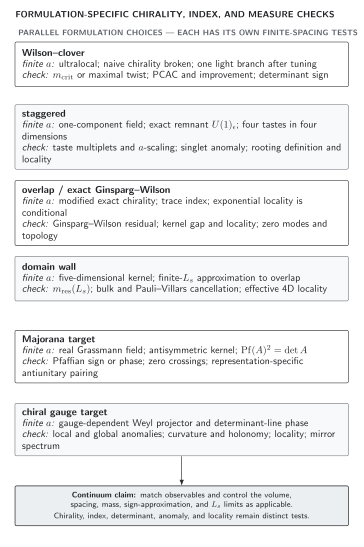
Lattice-fermion formulations trade different finite-regulator structures. Wilson methods require tuning and improvement; staggered methods require taste restoration and a separately qualified rooting step; exact Ginsparg–Wilson and overlap methods require locality and index checks; finite-$L_s$ domain-wall methods add a residual-mass test; Majorana and chiral-gauge targets add Pfaffian or Weyl-measure phases. The map is schematic, not to scale, and does not rank cost or accuracy.

A reproducible control sequence

Before accepting an overlap or domain-wall observable, require:

Observable-level validation checklist.

1. Kernel declaration: $D_{\mathrm W}$, $\rho$ or domain-wall height, boundary conditions, and the measured low spectrum of $H_{\mathrm W}$ or $H_T$.
2. Approximation declaration: sign or transfer approximation, spectral interval, deflation policy, and a uniform or measured error bound.
3. Algebra: gamma-five Hermiticity, $\lVert R_{\mathrm{GW}}\rVert$, spectral-circle deviation, and the trace index.
4. Locality: $f_N(r)$ at several volumes and a fit range that excludes periodic wraparound.
5. Fifth dimension: $L_s$ sequence, $m_{\mathrm{res}}$, $\Delta_{L_s}$, and Pauli–Villars bulk cancellation.
6. Topology: index agreement with an admissible background charge and explicit treatment of kernel crossings.
7. Observable: a renormalized Ward identity or spectrum compared at matched parameters with another formulation and then extrapolated in $a$ and volume.

Adversarial failure. A rational sign approximation may have a $10^{-12}$ maximum error on $[0.1,1]$ while the gauge ensemble contains kernel eigenvalues at $10^{-4}$. The quoted tolerance does not cover the actual spectrum; locality, the index, and residual chirality can all fail. The stop rule is to measure or rigorously bound the spectral interval before accepting the approximation error.

You should now be able to (1) derive the overlap Ginsparg–Wilson relation from the Hermitian kernel sign and (2) certify a finite-$L_s$ domain-wall calculation using independent locality, sign-approximation, overlap-matching, residual-mass, topology, and Ward-identity tests.

Exercises

Derive the overlap relation

Let $D=(1/\bar a)(1+V)$ with $V^\dagger V=1$ and $V^\dagger=\gamma_5V\gamma_5$. Show that $D$ obeys the Ginsparg–Wilson relation.

Solution

The Hermiticity condition gives $V\gamma_5V=\gamma_5$. Therefore

$$\bar aD\gamma_5D =\frac1{\bar a}(1+V)\gamma_5(1+V) =\frac1{\bar a}(2\gamma_5+V\gamma_5+\gamma_5V),$$

which equals $\gamma_5D+D\gamma_5$.

Estimate a finite-$L_s$ defect

For $h=1/2$, compute $1-\varepsilon_{L_s}(h)^2$ at $L_s=4$ and explain the limiting trend.

Solution

$\operatorname{artanh}(1/2)=\tfrac12\ln3$, so

$$1-\varepsilon_4(1/2)^2 =\operatorname{sech}^2(2\ln3) =\frac{4}{(9+1/9)^2} =\frac{324}{6724}\simeq0.0482.$$

At fixed nonzero $h$, the argument grows linearly with $L_s$ and the defect falls exponentially. The estimate is not uniform as $h\to0$.

Precise continuations

Anomalies, Ward Identities, and Chiral Diagnostics turns the index, $m_{\mathrm{res}}$, and currents into an interacting validation program. Fermion Determinants, Pfaffians, and Measure Positivity treats the resulting vectorlike measures. Theorem-level locality belongs to Chiral Gauge Theories and Standard Model Construction.

References

• Furman, Vadim, and Yigal Shamir. “Axial Symmetries in Lattice QCD with Kaplan Fermions.” Nuclear Physics B 439 (1995): 54–78. DOI.
• Hernández, Pilar, Karl Jansen, and Martin Lüscher. “Locality Properties of Neuberger’s Lattice Dirac Operator.” Nuclear Physics B 552 (1999): 363–378. DOI. Open PDF.
• Kaplan, David B. “A Method for Simulating Chiral Fermions on the Lattice.” Physics Letters B 288 (1992): 342–347. DOI. Open PDF.
• Neuberger, Herbert. “Exactly Massless Quarks on the Lattice.” Physics Letters B 417 (1998): 141–144. DOI. Open PDF.
• Shamir, Yigal. “Chiral Fermions from Lattice Boundaries.” Nuclear Physics B 406 (1993): 90–106. DOI. Open PDF.