Exponential Finite-Volume Effects

Exponential finite-volume corrections arise when a massive excitation must propagate around a spatial cycle and no intermediate state can go on shell. Their exponent is set by the nearest allowed singularity—often the lightest exchange mass, but sometimes a binding momentum or a more complicated kinematic scale—and their coefficient depends on the observable, boundary condition, and forward amplitude. The expectation fails for massless exchange, long-range interactions, open scattering states, thresholds, and boxes too small to order the image expansion.

Required background. Finite Volume as a Controlled Deformation supplies the range, mass-gap, temporal-wrap, and limit-order tests used here.

Helpful background. Asymptotic Scales, Remainders, Uniformity, and Optimal Truncation clarifies what a leading asymptotic term does and does not bound. Poles, Cuts, Thresholds, and Stable Particles supplies the singularity language that fixes the exponent.

Massive images in a periodic box

Work first with the three-dimensional Euclidean Green function

$$(-\nabla^2+m^2)G_\infty(\mathbf x)=\delta^{(3)}(\mathbf x), \qquad G_\infty(r)=\frac{e^{-mr}}{4\pi r}, \qquad m>0.$$

Massive finite-volume regime. Exponential image counting applies only after the nearest allowed singularity, the state type, spatial boundary condition, and treatment of Euclidean-time wrapping have been fixed.

The detailed choices are:

Field	Choice used on this page
Geometry	Cubic spatial box of side $L$ with periodic boundaries; Euclidean time is noncompact in the analytic benchmark
Image sum	$G_L(\mathbf x)=\sum_{\mathbf n\in\mathbb Z^3}G_\infty(\lvert\mathbf x+L\mathbf n\rvert)$
Expansion parameter	The relevant product is $\mu L$, where $\mu$ is derived from the nearest allowed singularity; it is not assigned automatically as the external mass
State restriction	A “mass shift” refers only to an isolated stable pole, or to a bound state with its binding scale stated
Remainder claim	The first omitted image shell is displayed; no fitted leading term is called an error bound without a bound on later shells and other scales

Periodizing the Green function gives

$$G_L(\mathbf x)= \sum_{\mathbf n\in\mathbb Z^3} \frac{e^{-m\lvert\mathbf x+L\mathbf n\rvert}} {4\pi\lvert\mathbf x+L\mathbf n\rvert}.$$

At the origin, subtracting the infinite-volume singular term leaves the exact image series

$$\Delta G_L(0)= \sum_{\mathbf n\ne\mathbf0} \frac{e^{-mL\lvert\mathbf n\rvert}} {4\pi L\lvert\mathbf n\rvert}.$$

Grouping integer vectors by length produces the checked asymptotic benchmark

$$\Delta G_L(0)= \frac{1}{4\pi L} \left[ 6e^{-mL} +\frac{12}{\sqrt2}e^{-\sqrt2mL} +\frac{8}{\sqrt3}e^{-\sqrt3mL} +3e^{-2mL}+\cdots \right].$$

The multiplicities $6,12,8,6$ count the vectors with squared lengths $1,2,3,4$; the length-$2$ shell contributes $6/2=3$. This independently checks the sign, dimensions, and leading coefficient. Twisted boundaries multiply each image by $e^{i\mathbf n\cdot\boldsymbol\theta}$, so the nearest images can cancel without changing the mass scale. Rectangular boxes replace $L\lvert\mathbf n\rvert$ by $\sqrt{\sum_i n_i^2L_i^2}$.

The relativistic four-dimensional Euclidean scalar propagator makes the power prefactor explicit:

$$D_\infty(r)=\frac{m}{4\pi^2r}K_1(mr) \sim \frac{\sqrt m}{4\sqrt2\,\pi^{3/2}r^{3/2}}e^{-mr} \left[1+O\!\left((mr)^{-1}\right)\right].$$

Thus “exponential” does not mean a pure $Ae^{-mL}$ fit. Algebraic prefactors, image multiplicities, twists, and subleading exponents are part of the prediction.

From an image to a stable-state correction

For an interacting observable $O$, Poisson summation converts the finite-volume loop correction into a sum of Fourier images. Moving the integration contour toward the nearest singularity gives the structural form

$$\Delta O(L) =\sum_{\mathbf n\ne0} C_{\mathbf n}(L)e^{-\mu_{\mathbf n}L} +\mathcal R(L),$$

where $C_{\mathbf n}$ contains algebraic powers of $L$ and on-shell residues or forward amplitudes. The contour displacement is allowed only when no singularity pinches it. Lüscher’s stable-particle analysis makes this statement precise and relates the leading mass shift to infinite-volume forward scattering data (Lüscher 1986, §§ 2–4, pp. 181–201); a later finite-size mass-shift treatment makes the pole and wrapping contributions explicit in Koma and Koma 2005, §§ 2–3.

Three qualifications are essential.

1. Stable external pole. If the target can decay, its finite-volume levels are real mixtures of multi-particle states, not a shifted complex resonance energy. Use a quantization condition and continue the resulting amplitude.
2. Correct wrapping scale. For a compact one-particle state the leading scale may be the lightest exchanged mass. For a shallow two-body bound state, a constituent can wrap with scale set by the binding momentum $\kappa$; typically the leading behavior is proportional to $e^{-\kappa L}/L$ up to kinematic and asymptotic-normalization factors.
3. Uniform distance from thresholds. When a denominator approaches an on-shell pinch, a coefficient can become enhanced and a nominally subleading term can compete. The asymptotic expansion is not uniform across the threshold.

Boundary conditions also change coefficients. A field with twist $\boldsymbol\theta$ has a nearest-image factor

$$\sum_{\lvert\mathbf n\rvert=1} e^{i\mathbf n\cdot\boldsymbol\theta} =2\sum_{i=1}^3\cos\theta_i.$$

For $\boldsymbol\theta=(\pi/2,\pi/2,\pi/2)$ the entire length-one shell cancels. The length-$\sqrt2$ and length-$\sqrt3$ shells cancel as well, while the length-$2$ shell has phase sum $2\sum_i\cos(2\theta_i)=-6$ and is the first nonzero image shell. This is an analytic check, not permission to ignore other twist-dependent physics.

A controlled fitting contract

A stable-particle or bound-state extrapolation should state:

• the pole or state whose shift is fitted, and the evidence that it is isolated;
• the candidate wrapping particles and why their quantum numbers allow the image;
• the derived exponent $\mu$, the algebraic power, image multiplicity, and boundary phase;
• the minimum fitted $\mu L$ and the relative size of the first omitted image shell;
• whether $a$, quark masses, couplings, $T$, and aspect ratios are matched across volumes; and
• alternative fits that add the next image, change the minimum volume, and use an independently constrained coefficient when available.

For the Yukawa benchmark, the ratio of the complete length-$\sqrt2$ shell to the length-$1$ shell is

$$r_{\sqrt2/1}=\sqrt2\,e^{-(\sqrt2-1)mL}.$$

It is about $0.270$ at $mL=4$ and $0.118$ at $mL=6$. A one-exponential fit at $mL=4$ therefore omits a geometrically fixed contribution at the tens-of-percent level even before dynamics changes the coefficients.

Adversarial failure. Three points can fit $Ae^{-mL}$ with a tiny $\chi^2$ even when a massless exchange contributes $B/L$. Over a short interval, the two smooth functions may be nearly collinear. Adding a larger volume, changing the boundary phase, or fitting the theoretically required power term is a physics test; goodness of fit alone cannot establish a mass gap.

The shared spectrum-to-amplitude map marks the boundary of the present result. Stable one-particle image corrections enter upstream of scattering quantization; they do not by themselves convert a box level into an infinite-volume amplitude.

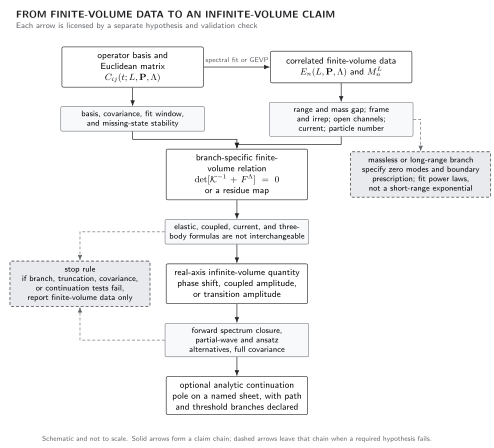
Finite-volume information reaches an infinite-volume claim only through a branch-specific map. Solid arrows show the controlled chain; dashed arrows show the long-range alternative and the stop rule. The image is schematic, not to scale, and the displayed determinant is structural: its channel, irrep, partial-wave, normalization, and sign conventions must be fixed locally.

Observable-level validation

Accept an exponential correction only after checking that:

• the target is a stable pole or a bound state with $\kappa$ and breakup thresholds stated;
• all lighter exchanges allowed by the observable’s quantum numbers have been considered;
• $R/L$, $\mu L$, $m_{\rm gap}T$, and the first omitted image ratio are reported;
• the predicted boundary-phase and box-shape dependence is visible within uncertainty;
• at least two fit windows in $L$ and one additional image term give compatible infinite-volume results; and
• a massless, on-shell, or threshold alternative is rejected by an observable-level test rather than by assumption.

What you can now do

You can now (1) derive the length-one and length-$\sqrt2$ image contributions, including their multiplicities and twist phases, for a massive propagator, and (2) decide from $R/L$, $\mu L$, threshold distance, and omitted-shell ratios whether a proposed leading-exponential correction is controlled.

Massless Fields, Long-Range Forces, and Finite-Volume QED treats the power-law branch. Elastic Two-Body Quantization Conditions treats the on-shell two-particle power laws.

Exercises

1. Count the next shell. Show that the squared-length-$5$ image shell has multiplicity $24$, and write its contribution to $\Delta G_L(0)$.

Solution

The vectors are permutations of $(\pm2,\pm1,0)$. There are $3! = 6$ permutations and $2^2=4$ independent signs, hence $24$ vectors. Their contribution is $24e^{-\sqrt5mL}/(4\pi\sqrt5L)$.

2. Test the asymptotic range. At what value of $mL$ does the complete length-$\sqrt2$ shell fall below $5\%$ of the length-$1$ shell in the Yukawa benchmark?

Solution

Solve $\sqrt2e^{-(\sqrt2-1)mL}<0.05$. This gives $mL>\log(\sqrt2/0.05)/(\sqrt2-1)\simeq8.07$. The exercise shows why “$mL\gtrsim4$” is not a universal precision criterion.

References

• Koma, Yoshiaki, and Miho Koma. “On the Finite Size Mass Shift Formula for Stable Particles.” Nuclear Physics B 713 (2005): 575–597. DOI. Open PDF.
• Lüscher, Martin. “Volume Dependence of the Energy Spectrum in Massive Quantum Field Theories. I. Stable Particle States.” Communications in Mathematical Physics 104 (1986): 177–206. DOI.