

Algorithm Validation and Ensemble Provenance
An ensemble generator is certified by demonstrating that its implemented transition preserves the declared finite-regulator target, reaches its relevant support, and survives exact-reference and deliberately broken tests. A long chain, high acceptance, plausible histograms, or short autocorrelation cannot establish these properties. Certification therefore begins before production: write the complete kernel contract, verify its algebraic hypotheses, compare independent implementations with exact small systems, and bind every generated configuration to an immutable record of target, code, randomness, and algorithm parameters.
Required background. Local, cluster, and global update families supplies proposal, conditional, and collective-kernel invariance arguments. Hybrid Monte Carlo and symplectic molecular dynamics supplies the reversibility, volume-preservation, and acceptance contract for trajectory proposals.
Helpful background. Pseudofermions, determinant ratios, and solver bias supplies the numerical-accuracy conditions for dynamical-fermion targets.
The complete generator contract
Section titled “The complete generator contract”Write the target first:
including regulator geometry, boundary conditions , bare parameters , reference measure , constraints, and support. Then write one transition step as an ordered composition of random draws and deterministic maps. Every branch—including rejection, solver failure, boundary handling, and exceptional floating-point path—belongs to the implemented kernel.
Local regulator and convention card. Finite-state kernels use row convention . Continuous residuals are evaluated against normalized quadrature or analytic moments. HMC reversibility is tested for with the same arithmetic, tolerances, and branch rules used in generation. The primary continuous fixture is a two-site real scalar with one undirected link, , , and ; its moments are computed by independently converged tensor-product quadrature.
A generator record answers the following questions without referring to future chain behavior.
- Target: What density and reference measure are invariant? Does a determinant sign, Jacobian, constraint, or boundary term enter?
- Proposal: What random variables are drawn, with what density and support? What deterministic transformation follows?
- Correction: Which acceptance, conditional, reweighting, or exact-refresh identity establishes stationarity?
- Geometry: Is the deterministic map reversible? What is its Jacobian or preserved area form?
- Numerics: Which solver, rational approximation, precision, and stopping rule enter the force and endpoint target?
- Coverage: What moves connect sectors, and which quantities are deliberately conserved?
- Schedule: How are component kernels composed, randomized, or adapted? Is adaptation frozen before the certified production interval?
The proof can use detailed balance, a direct stationarity equation, or composition of invariant kernels. If detailed balance is not intended, test the correct stationarity identity rather than declaring nonzero probability current a failure. General-state-space convergence still needs irreducibility and recurrence hypotheses; Tierney 1994, §§2–3 gives a careful formulation.
The reverse-density construction of Hastings 1970, pp. 97–109 supplies the local-proposal template, while Duane et al. 1987, pp. 216–222 supplies the reversible, volume-preserving trajectory template. Certification tests the implemented instance of either argument.
Correctness gates before performance
Section titled “Correctness gates before performance”The diagram below organizes the order of evidence. Inspect the two exits from the exactness gate: only the invariant branch proceeds to coverage and performance. The lower semantic matrix preserves every relationship in text.
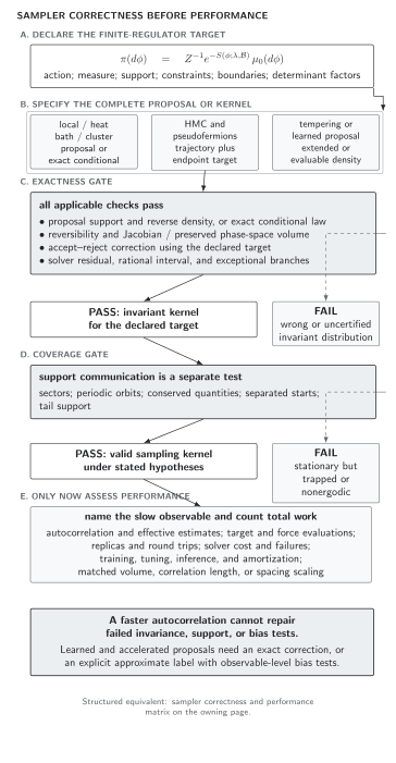
Correctness precedes efficiency for lattice-field samplers. A proposal or molecular-dynamics map reaches an invariant kernel only after its support, reverse probability or conditional law, Jacobian and reversibility where required, accept–reject correction, and solver or target evaluation pass. Ergodicity is a separate gate; autocorrelation, scaling, and training cost become meaningful only afterward. Original schematic, not to scale.
The logic has two independent axes. A kernel can be exact but inefficient, such as a very small local proposal. It can be fast but wrong, such as an uncorrected learned distribution with a support hole. No favorable entry in a performance column changes a failed correctness entry.
Sampler correctness and performance matrix
Section titled “Sampler correctness and performance matrix”The table is the structured equivalent of the figure and a template for a concrete run record. “Conditional” entries mean the stated algebraic representation must hold for the target; they are not universal guarantees.
| Kernel or estimator | Target and support | Proposal or conditional | Exact correction | Reversibility and Jacobian | Solver or approximation | Coverage and slow mode | Exact and bias tests | Performance report |
|---|---|---|---|---|---|---|---|---|
| Single-site Metropolis–Hastings | Declared positive lattice weight; proposal must cover every required local change | Local | Full Hastings ratio, including reverse proposal | Not required beyond the explicit reverse density; deterministic submaps need their Jacobian | Action differences evaluated to certified accuracy | Prove communication under the complete sweep; local critical modes may be slow | Enumerated transition matrix; exact moments; inject a missing proposal ratio or boundary term | Action evaluations, acceptance by region, slow observable, cost per effective estimate, volume and scaling range |
| Exact heat bath or Gibbs step | Target with a tractable normalized conditional | Draw | Conditional normalization; no rejection | Random draw need not be reversible as a map; kernel balance follows from the conditional | Conditional sampler and normalization must be exact or explicitly corrected | Composition of conditionals must connect the support | Enumerate a small lattice; compare conditional frequencies; inject a wrong local field | Conditional-draw cost, sweep definition, observable autocorrelation, scaling |
| Swendsen–Wang or Wolff cluster | Ferromagnetic spin target or another proven positive cluster representation | Auxiliary bonds with the model-specific activation law; flip full or seeded clusters | Exact alternating conditionals or boundary growth-ratio proof | Cluster flip is an involution; bond randomness supplies the reverse path | No linear solve; bond probabilities must remain valid probabilities | Check ergodicity and conserved sectors; clusters target collective order-parameter modes | Exact small-spin matrix; omit a periodic bond or apply the rule to frustration as negative controls | Activated bonds and flipped sites, cluster-size distribution, observable-specific cost and scaling |
| Overrelaxation plus stochastic refresh | Target whose conditional energy admits a measure-preserving reflection | Deterministic reflection composed with heat bath or Metropolis | Each factor preserves the same target | Reflection must be involutive with unit Jacobian; ordered composition may be nonreversible | Reflection center and local action evaluated consistently | Refresh step must break energy surfaces and periodic orbits | Conditional-energy invariance; remove refreshment and compare separated starts | Reflection and refresh costs separately; slow observable and composition ratio |
| Scalar or gauge HMC | Positive differentiable target on Euclidean fields or the correct group cotangent bundle | Gaussian momentum plus finite symplectic trajectory | Endpoint for a reversible unit-Jacobian proposal | Measure and verify volume or symplectic preservation | Force and endpoint accuracy stated separately | Momentum refresh and trajectory scheme must connect modes or sectors | Gaussian rational fixture; force finite differences; inject a missing half-kick, nonunit scaling, or asymmetric stopping | Force evaluations, acceptance, signed , reversal outliers, cost per effective observable, scaling |
| Positive-determinant pseudofermion HMC | Exact positive determinant factor and certified spectral support | Gaussian pseudofermion refresh plus HMC trajectory | Exact endpoint determinant action or controlled correction | HMC conditions plus deterministic solver behavior under reversal | True residuals, rational interval and maximum error, force and endpoint tolerances | Gauge-field kernel must traverse relevant sectors; determinant positivity does not imply coverage | Direct small-matrix determinant and force; inject interval excursion, stale solve, or loose endpoint action | Matrix applications, iterations, precision, failures, acceptance, slow observable, total cost |
| Parallel tempering or extended ensemble | Product of declared replica targets on a common state space | Within-replica kernels plus neighboring swaps | Exact swap ratio between replica weights | Swap is an involution with unit discrete Jacobian | Target evaluations at both replica parameters | Require replica round trips and cold-target sector visits | Enumerate a two-sector ladder; omit one replica factor as a negative control | All-replica cost, swap profile, round trips, cold-observable autocorrelation, scaling |
| Exactly corrected learned independence proposal | Declared target and normalized evaluable with common support | from an invertible or otherwise density-evaluable model | Independence Metropolis ratio | Change-of-variables Jacobian and reverse density must be accurate | Density, Jacobian, precision, model version, and any target surrogate recorded | Probe support and sector transfer; training data can hide modes | Exact small target; normalization and Jacobian tests; inject a support hole or remove correction | Training, tuning, target calls, inference, acceptance, failures, amortization horizon, matched scaling |
| Multilevel conditional estimator | Same parent target with a proven local subdomain factorization | Nested conditional samples at fixed boundary fields | Exact conditional recombination; not by itself a new global kernel | Subdomain updates obey their own transition contracts | Inner-solve and factorization approximations controlled | Does not establish faster global mixing | Small-volume direct expectation; vary inner samples and boundaries; break a factorization term | Parent-chain cost plus every inner update, variance reduction for the named observable, geometry and separation |
For each concrete application, replace generic phrases with measured values and explicit pass/fail thresholds. Acceptance and autocorrelation columns remain descriptive until the invariant, coverage, and bias columns pass.
Exact references and independent kernels
Section titled “Exact references and independent kernels”Validation should ascend from algebra to physics without skipping levels.
Finite discrete target. On the periodic four-spin Ising ring, enumerate the sixteen weights and every transition probability. Compute row sums, minimum matrix entry, the stationarity residual , and, for a reversible kernel, the balance tensor
Use both the exact bond correlation and an orbit-sensitive observable. A global-flip-only chain is the required example that passes stationarity but fails coverage.
Analytic continuous target. For a unit Gaussian, reproduce the one-step leapfrog map, unit determinant, exact , and acceptance at the fixture point on the HMC page. Numerically integrate the transition applied to Gaussian test functions and verify invariance.
Interacting scalar target. At fixed , compute the two-site normalization and even moments by tensor quadrature, doubling the order and domain until changes fall below a declared tolerance. Generate two ensembles: one with random-walk Metropolis and one with HMC using independently written action and force paths. Require agreement with quadrature and with each other for , , , and a tail probability such as . The tail test prevents low moments from hiding support failure.
Independence means more than changing a seed. Prefer separate transition families, separate derivative code, or direct quadrature. Shared action parsing and boundary indexing can otherwise reproduce the same defect in both chains.
Required injected defects
Section titled “Required injected defects”A validation suite that has never been shown to fail is not calibrated. Introduce one defect at a time and predict which check should respond.
- Action-sign defect: accept with in a Metropolis branch. Exact moments and must fail.
- Jacobian defect: scale one HMC coordinate without including its determinant. The volume check and continuous target moments must fail even if acceptance remains high.
- Solver defect: loosen only the endpoint pseudofermion solve or reuse a stale solution. Tolerance stability, reversibility, or direct determinant comparison must fail.
- Reversibility defect: remove the final half-kick or stop by a forward-only condition. and the symmetry diagnostics must respond.
- Support defect: restrict proposals or training data to one symmetry sector. Cross-start and tail or sector observables must disagree while within-sector acceptance may look excellent.
- Boundary defect: evaluate the target periodically but update as if an edge bond were absent. Exact discrete stationarity or scalar quadrature comparison must fail.
Record the magnitude at which each defect becomes detectable. This establishes sensitivity without pretending that an undetected smaller defect is absent; tolerance extrapolation supplies the latter control.
Immutable ensemble identity
Section titled “Immutable ensemble identity”The ensemble identity is fixed at generation time. A minimal record contains:
- action name and full parameters; geometry; boundary conditions; field representation; determinant powers; normalization-relevant conventions;
- ordered kernel schedule; proposal parameters; integrator and step sequence; force, acceptance, and solver tolerances; rational coefficients and spectral interval;
- source revision, dirty-tree marker, build recipe, compiler and numerical-library versions, executable hash, input-file hash, and runtime precision;
- random-number algorithm and version, master seed, stream or counter allocation, replica mapping, and restart policy;
- trajectory or update ranges, save cadence, acceptance decisions or sufficient restart state, warm-start source, and any discarded generation interval;
- configuration format and endianness where relevant, per-file checksums, ordered manifest checksum, completion state, and documented gaps or regenerations.
Derived observables, resampling choices, fit ranges, and autocorrelation estimates may evolve without changing the ensemble identity; they receive their own analysis record linked to the immutable configuration checksums. Generator correctness is the subject here. Equilibration assessment, stationarity tests on the realized chain, autocorrelation windows, covariance estimation, drift, and final uncertainty belong to Chapter 6.
Observable-level validation checklist
Section titled “Observable-level validation checklist”- Freeze the full target and implemented transition contract before production; include failure branches and adaptation rules.
- Prove stationarity, then separately test support communication, periodicity, conserved quantities, reversibility, Jacobians, and numerical accuracy as applicable.
- Pass an enumerated discrete target, an analytic continuous fixture, and an interacting small-system comparison using independent methods.
- Run all six injected defects and record which quantitative threshold detects each one.
- Compare multiple starts and independent kernels on observables sensitive to energy, symmetry, tails, and sectors.
- Bind every configuration to the immutable generation record and verify file and ordered-set checksums after transfer.
- Begin performance claims only after correctness passes; send realized-chain uncertainty and diagnostic choices to Chapter 6.
Learning outcomes
Section titled “Learning outcomes”After completing this page, you should be able to:
- write and verify a complete generator-level acceptance and invariance contract, including support, reversibility, Jacobian, solver, and exceptional-path conditions; and
- design an exact-reference suite that detects injected sign, Jacobian, solver, reversibility, support, and boundary defects while preserving an immutable ensemble identity.
Exercises
Section titled “Exercises”1. Design a boundary negative control. For the four-spin Ising ring, omit the bond from the local energy difference while retaining it in the target. Identify the smallest exact check that proves the kernel is wrong.
Solution
Enumerate the sixteen configurations and construct the transition matrix using the defective acceptance. The normalized target still includes all four bonds. Computing is sufficient: at , at least the states whose proposed flip changes the omitted bond have nonzero residual. A sampled mean is unnecessary and less sensitive.
2. Separate an exactness test from a chain diagnostic. Classify each quantity as generator-level, realized-chain inference, or both: , , split-chain mean difference, integrated autocorrelation time, and exact-moment agreement.
Solution
and are generator-level. Split-chain means and estimated integrated autocorrelation time are realized-chain diagnostics handled in Chapter 6. Exact-moment agreement is both: it validates the generator against a reference and, in finite samples, requires a correlated uncertainty analysis. It cannot replace the algebraic checks.
References
Section titled “References”- Duane, S., Kennedy, A. D., Pendleton, B. J., and Roweth, D. (1987). “Hybrid Monte Carlo.” Physics Letters B 195(2), 216–222. doi:10.1016/0370-2693(87)91197-X.
- Hastings, W. K. (1970). “Monte Carlo sampling methods using Markov chains and their applications.” Biometrika 57(1), 97–109. doi:10.1093/biomet/57.1.97.
- Tierney, L. (1994). “Markov chains for exploring posterior distributions.” The Annals of Statistics 22(4), 1701–1762. doi:10.1214/aos/1176325750.