

Reweighting, Taylor Expansion, and Imaginary Density
Reweighting, Taylor expansion, and simulations at imaginary chemical potential are three ways to infer a common real-density observable from a tractable neighborhood. Reweighting is an exact ratio identity but can lose overlap; Taylor expansion is local and can be defeated by noisy high derivatives or nearby complex singularities; imaginary-density continuation is sign-free in common cases but is an inverse problem constrained by analyticity and periodicity. Agreement is meaningful only inside a demonstrated common domain.
Required background. Anatomy and severity of a sign problem supplies phase and overlap diagnostics. Branches, sheets, continuation, and monodromy supplies analytic-domain control.
Helpful background. Estimators, covariance, and resampling supplies ratio covariance and correlated fitting.
Three estimators for one analytic target
Section titled “Three estimators for one analytic target”Convention and regulator card. Fix lattice spacing, volume, masses, temperature, action, and observable definition. Let and choose a reference ensemble at , usually zero or imaginary. All formulas concern this fixed finite regulator. A later continuum claim requires repeating the complete inference at several lattice spacings.
For a measure and observable ,
This reweighting identity is exact when the target measure is absolutely continuous with respect to the reference and both integrals exist. Its delta-method variance depends on the covariance of and :
A small denominator, heavy-tailed , or missing target support invalidates naive Gaussian errors. Histogram reweighting was formulated as a way to move between nearby ensembles Ferrenberg and Swendsen 1988, pp. 2635–2636; “nearby” is an overlap condition, not merely a small coordinate distance.
If is analytic at zero,
Charge-conjugation symmetry makes even for charge-even observables. Derivatives contain connected combinations of observable derivatives and derivatives of ; they must be estimated jointly because their cancellations are correlated. Early finite-density lattice calculations made this derivative structure explicit Allton et al. 2002, § II, Eqs. (4), (7)–(14).
At imaginary density ,
for an even observable. One fits symmetry-allowed functions on imaginary points, then evaluates the same analytic function at real . In QCD, center symmetry also imposes a periodic structure and nonanalytic boundaries; an early lattice-QCD study with imaginary chemical potential explicitly restricted continuation to an analytic interval de Forcrand and Philipsen 2002, §§ 2–3, Eqs. (4), (7), (14)–(15).
Truncation and analytic-domain diagnostics
Section titled “Truncation and analytic-domain diagnostics”At finite volume, the partition function is often a polynomial or convergent Laurent series in fugacity, so its zeros are isolated in the complex plane. Observables derived from are singular at the nearest zero. In the thermodynamic limit, zeros may accumulate into cuts or phase boundaries. The Taylor radius is therefore bounded by
where are singularities on every relevant sheet. Finite-order ratios such as
are diagnostics, not guaranteed radius estimators before asymptotic behavior is established. Correlated coefficient errors and an accidentally small denominator can create false plateaus.
For a truncation at order , report at least three checks: stability after dropping the largest imaginary- points, stability under one higher/lower order, and out-of-sample prediction of points not used in the fit. A Padé or conformal ansatz may improve approximation, but its poles and mapping assumptions become additional systematic inputs.
Exact fixture and common observable
Section titled “Exact fixture and common observable”For the chapter fixture,
Use the density
as the common target.
- Reweighting: sample with and use in the ratio identity.
- Taylor: expand from exact or sampled derivatives at zero.
- Imaginary density: evaluate and fit its only allowed Fourier modes; continue .
The exact analytic singularities satisfy . Although no zero lies on the real axis for positive , complex zeros limit the Taylor series. This is a clean test that a sign-free imaginary interval does not authorize unlimited real continuation.
The correctness map locates the failure witness for each method. Follow a branch only after its condition has been checked.
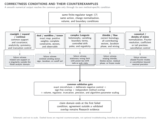
Each reformulation has a different correctness condition and a characteristic counterexample. Apparent numerical convergence is insufficient when overlap is absent, a dual sector or Jacobian is missing, complex-Langevin boundary terms survive, a contributing thimble is omitted, or canonical and density-of-states cancellations exceed resolved precision. The map is schematic and does not rank current algorithms.
Adversarial failure cases
Section titled “Adversarial failure cases”Correlated numerator and denominator analyzed separately. Propagating their errors as independent can greatly overstate or understate uncertainty. Resample the complete ratio using the same configurations.
A polynomial fits all imaginary points. If all points lie far inside the fit interval, many ansätze extrapolate smoothly but disagree at real . Reserve boundary points and compare symmetry-respecting alternative orders.
Coefficient-ratio plateau at low order. A few noisy coefficients are not asymptotics. Test the estimator on the exact fixture after injecting comparable covariance and examine complex zeros directly where possible.
Multiparameter reweighting hides support loss. Tuning a second coupling may improve histogram overlap for one bulk variable while the phase or an observable-specific sector remains unsampled. Report joint, not marginal, overlap diagnostics.
Observable-level validation checklist
Section titled “Observable-level validation checklist”- Carry the same normalized observable, charge convention, and regulator through all three methods.
- For reweighting, report phase, log-weight tails, covariance, effective support, and results from more than one reference ensemble.
- For Taylor expansion, publish the coefficient covariance matrix, symmetry zeros, order stability, and a complex-singularity diagnostic.
- For imaginary density, enforce exact periodicities, reserve validation points, vary the continuation ansatz, and identify the nearest known nonanalytic boundary.
- Demonstrate agreement in an overlap window and deliberate disagreement beyond at least one known method boundary.
- Repeat the full comparison with volume and lattice spacing before extending a physical claim.
Exercises
Section titled “Exercises”1. First coefficients of the fixture density
Section titled “1. First coefficients of the fixture density”Find the coefficients of and in .
Solution
Let . Expanding numerator and denominator,
The odd structure is fixed by charge conjugation.
2. Why an imaginary-axis fit can fail
Section titled “2. Why an imaginary-axis fit can fail”Give an analytic function whose first Taylor coefficients at zero agree with , yet differs at real while remaining arbitrarily close on a finite set of imaginary points.
Solution
Take
It has the same coefficients through order , and agrees exactly at the chosen imaginary points , but generally differs for real . Additional analytic assumptions and withheld points are therefore necessary.
Learning outcomes
Section titled “Learning outcomes”After working this page, you should be able to:
- Compute one finite-density observable by reweighting, Taylor coefficients, and imaginary-density continuation, including correlated uncertainty and truncation tests.
- Locate overlap loss, a nearby complex singularity, or continuation-model dependence and set the parameter boundary at which the inference must stop.
Related topics
Section titled “Related topics”When a local analytic neighborhood is insufficient, dual reformulations may give an exact positive representation for special models. The Research methods—complex Langevin, thimbles, and canonical or density-of-states reconstruction—each require their own correctness test. The finite-density method reliability matrix compares those tests field by field.
References
Section titled “References”- Allton, C. R., et al. “The QCD Thermal Phase Transition in the Presence of a Small Chemical Potential.” Physical Review D 66 (2002): 074507. doi:10.1103/PhysRevD.66.074507.
- de Forcrand, Philippe, and Owe Philipsen. “The QCD Phase Diagram for Small Densities from Imaginary Chemical Potential.” Nuclear Physics B 642 (2002): 290–306. doi:10.1016/S0550-3213(02)00626-0.
- Ferrenberg, Alan M., and Robert H. Swendsen. “New Monte Carlo Technique for Studying Phase Transitions.” Physical Review Letters 61 (1988): 2635–2638. doi:10.1103/PhysRevLett.61.2635.