

Gradient Flow, Flow Scales, and Renormalized Gauge Observables
Gauge-field gradient flow evolves a configuration into a smoother field at positive flow time . Local gauge-invariant composites built from the flowed field are finite after the underlying theory is renormalized, and dimensionless conditions on the flowed energy density define precise reference scales. Flow remains a scale-dependent transformation: its smoothing radius, lattice discretization, integration error, finite volume, and order of limits must be controlled.
Required background. Topology and lattice index diagnostics distinguishes sector information from a particular smoothed estimator, while gauge ensembles and renormalized observables supplies covariance and continuum controls.
Helpful background. Scale setting and nonperturbative operator renormalization explain how a flow scale or flowed operator enters a physical result.
Continuum and lattice flow equations
Section titled “Continuum and lattice flow equations”Local convention and regulator card. Use , flow toward positive by , and quote the smoothing radius as in four dimensions. State the simulation action, flow action, integrator and step, energy-density discretization, boundary conditions, , , and whether the continuum limit is taken at fixed positive physical before any small-flow-time limit.
For a continuum gauge field with , the Yang–Mills gradient flow is
up to an optional gauge-damping term that changes only the flow-time gauge. Since , the linearized equation is a heat equation. The field is averaged over a characteristic radius
in four dimensions.
For lattice links , a standard group-valued flow has the form
where is a chosen flow action and its Lie-algebra derivative. The simulation action, flow action, and discretization of a measured composite may all differ; their combination determines leading cutoff effects.
Numerically, confirm group unitarity, monotonic decrease of for the gradient convention, and convergence under flow-step refinement. These are necessary algorithmic checks, not substitutes for a continuum extrapolation.
The smoothing interpretation and reference-scale construction are developed in Lüscher 2010, §§ 2–3; the all-orders perturbative finiteness analysis is given in Lüscher and Weisz 2011, §§ 2–8.
Reference scales from the energy density
Section titled “Reference scales from the energy density”Let
The dimensionless condition
defines , while
defines . The conventional constant and all discretizations must be reported. These quantities are precise reference scales, not automatically physical observables; an experimentally known input or another accepted physical scale is still required to express them in conventional units.
Because and come from the same configurations as many target observables, their covariance should be retained in dimensionless ratios and continuum fits.
The flow window
Section titled “The flow window”A useful positive-flow-time observable requires scale separation,
or equivalently , with stronger numerical margins determined empirically. The left inequality suppresses discretization artifacts such as ; the right controls finite-volume distortion and avoids smearing around periodic boundaries.
A representative expansion is
Improved flow and observable choices can reduce but do not justify including points with . Window stability is tested by moving both endpoints and repeating the continuum fit.
Small-flow-time expansion
Section titled “Small-flow-time expansion”For a flowed renormalized composite ,
as , ordered by operator dimension and symmetries. The coefficients are a matching problem. A common controlled order is:
- take at fixed positive physical ;
- control or bound finite-volume effects;
- apply the matching relation and, if required, take within a stable window.
Taking at fixed collapses the smoothing radius onto the cutoff and invalidates the expansion. Identifying with a renormalization scale without computing the matching coefficients is likewise incomplete.
Flowed topology
Section titled “Flowed topology”At positive flow time, an improved field-strength charge often clusters near integers and definitions agree more closely. This makes flow a valuable diagnostic. Yet two questions remain separate:
- Does the charge definition approach the continuum topological observable?
- Did the Markov chain sample sectors with their equilibrium weights?
Flow may improve the first and cannot repair the second. Track charge histories before and after flow, state in physical units, and test definition and spacing dependence.
A complete flow result
Section titled “A complete flow result”Report the ensemble action, flow action, integrator and step, energy or operator discretization, , , , scale input, autocorrelation, and continuum model. The regime map emphasizes that the path from smoothing to a renormalized claim passes through both a flow window and a matching or reference-scale definition.
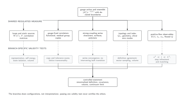
The positive-flow branch requires a scale-separation window, integration refinement, and matching before joining the final continuum claim. Smoothness alone is not sufficient. The diagram is schematic and not to scale.
Adversarial failure: a smooth diagonal path with unsuppressed cutoff error
Section titled “Adversarial failure: a smooth diagonal path with unsuppressed cutoff error”Take a sequence with at every spacing and observe that changes little. The configurations look smoother as the nominal decreases, yet
in physical units. The leading artifact never becomes small, so this diagonal path cannot establish the positive- continuum observable or its small-flow-time expansion. Fixed physical at several values, followed by a separate -window analysis, is the test that this apparently stable sequence fails.
Observable-level validation checklist
Section titled “Observable-level validation checklist”- Verify , link unitarity, gauge covariance, and monotonic flow-action decrease with the stated sign convention.
- Refine the integration step and require , , and to converge within the numerical error.
- Compare at least two flow or energy discretizations and fit their dependence at fixed positive physical .
- Move both ends of the window and repeat at another volume.
- Carry flow-scale covariance into the target ratio, and test matching-scale and small- stability only after the fixed- continuum limit.
Common pitfalls
Section titled “Common pitfalls”Calling flow “just cooling.” Gradient flow has a precise differential equation and supports renormalized positive- composites. That precision is lost if the action and integrator are unspecified.
Treating as harmless. Flow time is a physical resolution scale. Compare at fixed physical , not merely at equal .
Removing the cutoff and flow limits together without analysis. Terms such as make diagonal limit paths dangerous. Demonstrate a stable ordered or joint extrapolation.
Learning outcomes
Section titled “Learning outcomes”- Given a lattice flow prescription, compute or , verify integration and scale-separation conditions, and propagate the resulting reference-scale covariance into an observable.
- Given data over , , and , distinguish a finite positive-flow-time observable from arbitrary smoothing and design ordered continuum, volume, matching, and small-flow-time tests.
Exercises
Section titled “Exercises”- If is held fixed while , what happens to in physical units and to ?
Solution
, while remains finite. Cutoff effects are therefore not suppressed.
- A measured gives . Is this automatically inside the flow window?
Solution
No. The radius is only about , so one must test discretization dependence, and it must also be small compared with . The numerical window is an empirical scaling statement, not an algebraic threshold.
The chapter’s gauge convention table places the flow-time window and numerical refinement alongside the observable’s renormalization and continuum limits.
References
Section titled “References”- Lüscher, M. (2010). Properties and uses of the Wilson flow in lattice QCD. Journal of High Energy Physics, 2010(08), 071. DOI.
- Lüscher, M., and Weisz, P. (2011). Perturbative analysis of the gradient flow in non-Abelian gauge theories. Journal of High Energy Physics, 2011(02), 051. DOI.
Further reading
Section titled “Further reading”- Narayanan, R., and Neuberger, H. (2006). Infinite N phase transitions in continuum Wilson loop operators. Journal of High Energy Physics, 2006(03), 064. DOI.