The Wilson Gauge Action and Its Continuum Limit

The Wilson action is the simplest local gauge-invariant action for compact link variables. Its plaquette term reproduces the Yang–Mills kinetic term when fields vary slowly compared with the lattice spacing. That classical match fixes normalization, but a continuum quantum theory additionally requires a line of constant physics, increasing physical volume, and control of cutoff effects.

Required background. Use the orientation and trace conventions from links, plaquettes, and gauge invariance and the continuum-expansion discipline from scalar actions and difference operators.

Helpful background. Symanzik analysis and improvement explains how higher-dimension operators organize cutoff effects; the Yang–Mills action fixes the continuum target normalization.

Wilson’s finite-spacing action

Local convention and regulator card. Unless anisotropy is introduced explicitly below, use a four-dimensional isotropic hypercubic lattice with spacing $a$, periodic spatial boundaries, $G=SU(N)$, fundamental Hermitian generators satisfying $\operatorname{tr}(T^aT^b)=\delta^{ab}/2$, and one positively oriented plaquette for each unordered pair $\mu<\nu$. The bare normalization is $\beta=2N/g_0^2$; physical spacing, volume, and anisotropy are measured quantities, not inputs inferred from that formula alone.

On an isotropic $d$-dimensional hypercubic lattice, choose $SU(N)$ fundamental generators with $\operatorname{tr}(T^aT^b)=\delta^{ab}/2$. The Wilson action is

$$S_W[U]=\beta\sum_x\sum_{\mu<\nu} \left(1-\frac1N\operatorname{Re}\operatorname{tr}U_{\mu\nu}(x)\right), \qquad \beta=\frac{2N}{g_0^2}$$

in four dimensions. The partition function uses one normalized Haar measure per independent link,

$$Z=\int\prod_{x,\mu}dU_\mu(x)\,e^{-S_W[U]}.$$

Left- and right-invariance of Haar measure makes the integration measure exactly gauge invariant. The constant term is physically irrelevant but makes every plaquette contribution nonnegative because $\operatorname{Re}\operatorname{tr}U_p/N\le1$.

For other generator or trace conventions, $\beta$ changes. The equality $\beta=2N/g_0^2$ is therefore not a convention-free definition.

The plaquette action and its strong-coupling loop interpretation were introduced in Wilson 1974, pp. 2445–2459.

Recovering the continuum normalization

For smooth fields with

$$U_{\mu\nu}(x)=\exp\!\left[i a^2g_0F_{\mu\nu}^a(x)T^a+O(a^3)\right],$$

expand the trace. The linear term vanishes for $SU(N)$, and

$$1-\frac1N\operatorname{Re}\operatorname{tr}U_{\mu\nu} =\frac{a^4g_0^2}{4N}F_{\mu\nu}^aF_{\mu\nu}^a+O(a^6).$$

Using $a^4\sum_x\to\int d^4x$ and $\beta=2N/g_0^2$ gives

$$S_W\longrightarrow \frac12\int d^4x\sum_{\mu<\nu}F_{\mu\nu}^aF_{\mu\nu}^a =\frac14\int d^4x\,F_{\mu\nu}^aF_{\mu\nu}^a.$$

The two expressions agree because the second sum counts both $(\mu,\nu)$ and $(\nu,\mu)$. This factor-of-two check is a useful guard against mixing ordered and unordered plaquette sums.

The derivation establishes the classical target for smooth configurations. It does not show that an arbitrary bare coupling lies near the desired quantum continuum fixed point, nor that one lattice spacing is enough to identify the leading power of $a$.

The orientation diagram provides a direct normalization check: reverse the top and left links, telescope the site transformations, and only then expand the resulting closed product.

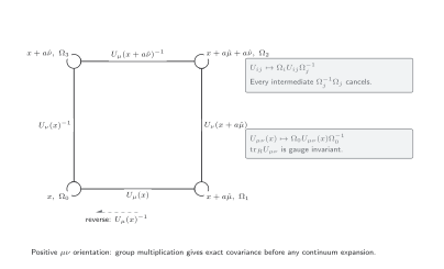
The positive $\mu\nu$ plaquette transforms by conjugation at its base point. Its trace is exactly invariant at finite spacing, while its interpretation as $\exp(ia^2g_0F_{\mu\nu}+\cdots)$ is asymptotic. The drawing is schematic.

Anisotropic lattices

With spatial spacing $a_s$ and temporal spacing $a_t$, spatial and temporal plaquettes carry distinct bare coefficients:

$$S=\frac{2N}{g_0^2}\left[ \frac{a_t}{a_s}\sum_{x,i<j}\left(1-\frac1N\operatorname{Re}\operatorname{tr}U_{ij}\right) +\frac{a_s}{a_t}\sum_{x,i}\left(1-\frac1N\operatorname{Re}\operatorname{tr}U_{0i}\right) \right]$$

at tree level. Quantum corrections renormalize the physical anisotropy $\xi_R=a_s/a_t$ away from its bare input. A measured dispersion relation, static-potential comparison, or other matching observable must tune $\xi_R$; inserting the bare ratio into all later conversions is not a controlled procedure.

Reflection positivity also constrains which extended loops and signs may be added to an action if a positive transfer-matrix interpretation is required. Classical $O(a^2)$ improvement alone does not guarantee that property.

The distinction between classical improvement and a positive transfer construction is explicit in Osterwalder and Seiler 1978, pp. 440–471 and Lüscher and Weisz 1985, pp. 59–77.

Cutoff expansion and continuum evidence

For a dimensionless renormalized observable $R$ along a line of constant physics, the Symanzik description has the form

$$R(a,L)=R_\star+c_1(a\Lambda)^p+c_2(a\Lambda)^{p'} +d_1e^{-mL}+\cdots,$$

possibly with logarithms. The leading $p$ depends on the action, observable, and symmetries. A valid continuum claim therefore specifies:

• which renormalized quantities are held fixed as $a$ changes;
• how the scale and renormalized anisotropy are determined;
• how large $mL$ is and whether volume effects are fitted or bounded;
• at least one alternative cutoff ansatz or improved discretization;
• stability under omitting the coarsest spacing.

The action’s approach to $F^2$ is one link in this chain, not the final result.

Worked normalization check for SU(2)

For $T^a=\sigma^a/2$, write $X=a^2g_0F^aT^a$. Since $\operatorname{tr}X=0$ and $\operatorname{tr}X^2=a^4g_0^2F^aF^a/2$,

$$\frac12\operatorname{Re}\operatorname{tr}e^{iX} =1-\frac14\operatorname{tr}X^2+O(X^4) =1-\frac{a^4g_0^2}{8}F^aF^a+O(a^8).$$

Thus $1-\frac12\operatorname{Re}\operatorname{tr}U_p=a^4g_0^2F^aF^a/8+\cdots$. Multiplication by $\beta=4/g_0^2$ produces $a^4F^aF^a/2$ for each unordered pair, exactly as required. If instead one uses anti-Hermitian generators or absorbs $g_0$ into $A_\mu$, both the exponential and $\beta$ relation must be translated together.

What the regime map prevents

The Wilson action supplies a probability measure, but it does not make gauge-fixed correlators unique, strong-coupling series valid at weak coupling, loop diagnostics equivalent, or flowed topology independent of $t$. Inspect the distinct dashed tests below before following any branch to a continuum statement.

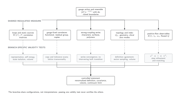
One regulated gauge measure feeds several nonequivalent inference branches. The action’s classical continuum expansion validates none of their estimator, regime, or limit tests automatically. The diagram is schematic and not to scale.

Adversarial failure: correct normalization on a false continuum sequence

Take lattices with $N_s=16,24,32$ at the same bare $\beta$, and merely relabel their nominal spacing as $a\propto1/N_s$. The plaquette expansion still reproduces $\frac14F^2$ algebraically on every lattice, while the path-integral measure is unchanged in lattice units: only the box contains more sites. A dimensionless mass ratio may look stable because the bare action is the same, but this tests finite volume rather than tuning the spacing. The classical coefficient test can therefore pass exactly while the claimed continuum extrapolation has no physical abscissa.

Observable-level validation checklist

• Apply independent site transformations and verify both the Haar measure and every plaquette term are unchanged.
• Evaluate a weak, constant commuting $SU(2)$ background and recover the coefficient $a^4F^a_{\mu\nu}F^a_{\mu\nu}/2$ for each unordered pair.
• Determine the renormalized anisotropy from a dispersion relation or matched spatial and temporal observable rather than substituting the bare ratio.
• Match at least one dimensionless renormalized quantity across three or more spacings, repeat at a second volume, and retain their covariance.
• Vary the cutoff ansatz or discretization and omit the coarsest spacing; a continuum result must remain stable within its stated uncertainty.

Common pitfalls

Treating the naive expansion as a quantum proof. The small-$a$ series identifies the classical continuum operator. A quantum continuum limit also needs renormalized tuning and scaling evidence.

Forgetting how pairs are counted. $\sum_{\mu<\nu}$ and $\sum_{\mu,\nu}$ differ by a factor of two for antisymmetric $F_{\mu\nu}$. State the sum before matching coefficients.

Equating bare and physical anisotropy. The coefficients above are tree-level values. Tune and report the renormalized anisotropy on interacting ensembles.

Learning outcomes

1. Expand the Wilson plaquette for a stated generator and pair-counting convention and recover the continuum Yang–Mills coefficient, including the anisotropic tree-level factors.
2. Given a proposed lattice sequence, decide from matched observables, volumes, and cutoff alternatives whether it constitutes continuum evidence or only a classical normalization check.

Exercises

1. Repeat the plaquette expansion for generators satisfying $\operatorname{tr}(T^aT^b)=T_F\delta^{ab}$ and derive the required four-dimensional $\beta$.

Solution

The plaquette term is $a^4g_0^2T_FF^aF^a/(2N)$. Matching $\frac12a^4F^aF^a$ for each $\mu<\nu$ gives $\beta=N/(g_0^2T_F)$, which reduces to $2N/g_0^2$ when $T_F=1/2$.

2. Why does agreement of one observable at two lattice spacings not determine $p$ in the cutoff expansion?

Solution

With unknown $R_\star$, coefficient, and exponent, two values underdetermine the model; volume effects and logarithms add further ambiguity. Multiple spacings plus theory-motivated alternative fits are required.

References

• Lüscher, M., and Weisz, P. (1985). On-shell improved lattice gauge theories. Communications in Mathematical Physics, 97, 59–77. DOI.
• Osterwalder, K., and Seiler, E. (1978). Gauge field theories on a lattice. Annals of Physics, 110, 440–471. DOI.
• Wilson, K. G. (1974). Confinement of quarks. Physical Review D, 10, 2445–2459. DOI.