Relativistic processes immediately expose a limitation of fixed-particle-number quantum mechanics. In neutron beta decay,
n⟶p+e−+νˉe,
one incoming neutron is replaced by a proton, an electron, and an antineutrino. Energy, momentum, electric charge, and the other exact charges remain conserved, but neither the particle species nor the total particle count is fixed. A relativistic quantum theory therefore needs a Hilbert space and operators that can connect sectors with different particle content.
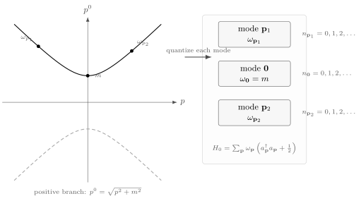
To build that language, begin with the simplest free case. A single massive neutral spin-zero bosonic field is a collection of positive-frequency harmonic oscillators, one for each allowed momentum. A single oscillator has a tower of states ∣0⟩,∣1⟩,∣2⟩,…; in field theory the integer np becomes the number of particles carrying momentum p.
This is not just a suggestive analogy. The relativistic energy of one spinless particle is
ωp=p2+m2,
and the energy of noninteracting particles is additive. The harmonic oscillator is precisely the quantum system whose spectrum is generated by adding identical bosonic quanta. The first construction in this course marries these facts: attach a harmonic oscillator to every momentum mode and let its quanta be particles.
The result is the seed of Fock space, perturbation theory, propagators, and scattering amplitudes. Interactions will later mix the modes, create particles, annihilate particles, and shift the location of poles, but the free oscillator basis is the table on which all those calculations are set.
A useful way to read this page is to separate two ideas that often get blended together. First, a harmonic oscillator has a rigorous algebra of creation, annihilation, and number operators. Second, a free relativistic scalar field assigns one such oscillator to each allowed momentum. The particles are the oscillator quanta; they are not extra objects added on top of the field. Fermionic fields require anticommuting creation and annihilation operators and will be treated separately.
Lorentz invariance fixes the invariant mass of a one-particle state by
pμpμ=m2.
On the positive-energy branch,
p0=ωp=p2+m2.
Measuring the one-particle and additive energies relative to the selected free vacuum, a one-particle momentum eigenstate satisfies
H∣p⟩=ωp∣p⟩,P∣p⟩=p∣p⟩.
For noninteracting particles, the Hamiltonian is additive. A state with momenta p1,…,pN has
H∣p1,…,pN⟩=(ωp1+⋯+ωpN)∣p1,…,pN⟩.
This formula has the same structure as a set of independent counters. For each momentum p, we only need to know how many times ωp appears in the total energy. That observation is the doorway from wave mechanics to fields.
For the free scalar field considered here, each allowed momentum p labels an oscillator with frequency ωp=p2+m2. Occupying that oscillator creates particles on the positive-energy mass shell.
For the bosonic scalar field considered here, “free field” therefore means a system whose normal modes are independent oscillators and whose mode frequencies are determined by relativistic kinematics. See Coleman 2019, § 2.2, pp. 20–21 for the occupation-number spectrum and its oscillator interpretation.
Start with one classical oscillator of positive frequency ω>0,
L=21q˙2−21ω2q2.
Its canonical momentum is
π=∂q˙∂L=q˙,
and the Hamiltonian is
H=πq˙−L=21π2+21ω2q2.
Canonical quantization promotes q and π to operators obeying
[q,π]=i.
Define ladder operators by
a=2ωq+2ωiπ,a†=2ωq−2ωiπ.
Equivalently,
q=2ωa+a†,π=−i2ω(a−a†).
Using [q,π]=i, the ladder operators obey
[a,a†]=1.
Substituting the inverse relations into the Hamiltonian gives
H=ω(a†a+21).
The constant ω/2 is the zero-point energy of this specified, unshifted quadratic Hamiltonian. It appears because a and a† do not commute; choosing another overall energy origin does not remove that algebraic term from the original Hamiltonian. For a field, summing these constants over an unbounded set of modes produces the ultraviolet vacuum-energy divergence.
Define the number operator
N=a†a.
Its commutators with the ladder operators are
[N,a†]=a†,[N,a]=−a.
So if
N∣n⟩=n∣n⟩,
then
N(a†∣n⟩)=(n+1)a†∣n⟩,N(a∣n⟩)=(n−1)a∣n⟩.
The eigenvalues of N are nonnegative, since
⟨n∣N∣n⟩=⟨n∣a†a∣n⟩=∥a∣n⟩∥2≥0.
Repeated lowering must therefore stop. The state where it stops is the oscillator vacuum,
a∣0⟩=0.
The normalized excited states are
∣n⟩=n!(a†)n∣0⟩,n=0,1,2,….
The operators act as
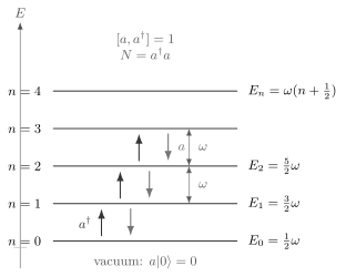
a†∣n⟩=n+1∣n+1⟩,a∣n⟩=n∣n−1⟩.
Thus
H∣n⟩=ω(n+21)∣n⟩.
The harmonic oscillator spectrum. The operator a† raises the occupation number by one and increases the energy by ω; the operator a lowers the occupation number by one and decreases the energy by ω.
In the basis ∣0⟩,∣1⟩,∣2⟩,…, the matrix elements are
The frequency of the oscillator labeled by p is the relativistic one-particle energy,
ωp=p2+m2.
Before subtracting its vacuum constant, the regulated quadratic free Hamiltonian is
Hfree=p∑ωp(ap†ap+21).
The vacuum energy is
Evac=21p∑ωp.
Without the ultraviolet cutoff, this sum already diverges at fixed L: along n=(j,0,0), the positive frequencies grow with ∣j∣. A finite box is not an ultraviolet regulator. At fixed finite cutoff the vacuum energy is finite; as V→∞ its total is extensive while its density has a finite thermodynamic limit. Removing the cutoff is a separate operation.
For the selected free vacuum on this fixed background, subtract the finite regulated constant to define the excitation Hamiltonian. The notation below means normal ordering the underlying unsimplified quadratic oscillator presentation, not applying colons to the already reduced expression ωp(Np+1/2) as though scalar constants disappeared:
:Hfree:=p∑ωpap†ap.
In subsequent field-mode formulas, Hfree without colons denotes this excitation Hamiltonian. The finite subtraction changes neither the energy gaps nor the creator commutators in the same background. In the continuum, the excitation Hamiltonian is defined directly on its operator domain, not by subtracting infinity from an operator; see the regulated Hamiltonian and vacuum constant. Choosing an energy origin in this fixed-background calculation does not settle gravitational or boundary-dependent vacuum-energy questions.
Before taking V→∞, it is worth keeping the finite-volume dictionary visible:
p∑⟶V∫(2π)3d3p,δpq⟶V(2π)3δ(3)(p−q).
Different continuum normalizations move factors of V and (2π)3 between ap, a(p), and ∣p⟩. The physics is unchanged, but the bookkeeping is not. This is why early calculations are safest in a box, and why later relativistic pages will state their state normalization explicitly.
The normalized occupation-number state is
∣{np}⟩=p∏np!(ap†)np∣0⟩,np=0,1,2,…,
where only finitely many occupation numbers are nonzero for an ordinary finite-particle state. It obeys
Np∣{nq}⟩=np∣{nq}⟩.
For the normal-ordered free Hamiltonian,
Hfree∣{np}⟩=(p∑npωp)∣{np}⟩,
while the momentum operator is
P=p∑pap†ap,
so
P∣{np}⟩=(p∑npp)∣{np}⟩.
The integer np is now a particle number: it counts how many quanta occupy the mode with momentum p.
The interpretation of ap† as a particle-creation operator follows from its commutators with conserved generators.
For the normal-ordered free Hamiltonian,
H=q∑ωqaq†aq,
we compute
[H,ap†]=q∑ωq[aq†aq,ap†].
Using [AB,C]=A[B,C]+[A,C]B and [aq†,ap†]=0,
[aq†aq,ap†]=aq†[aq,ap†]=aq†δqp.
Therefore
[H,ap†]=ωpap†.
Similarly,
[P,ap†]=pap†.
If ∣Ψ⟩ has energy E and momentum PΨ, then ap†∣Ψ⟩ has energy E+ωp and momentum PΨ+p, provided the resulting state is nonzero. This is the precise sense in which ap† creates one particle of momentum p: it shifts the eigenvalues of the conserved generators by the one-particle energy and momentum. This definition is more robust than picturing a particle as a tiny object being inserted into space.
The vacuum of the free field is the state annihilated by every lowering operator:
ap∣0⟩=0for every p.
A one-particle state is
∣p⟩=ap†∣0⟩,
and a two-particle state is
∣p,q⟩=ap†aq†∣0⟩.
If both particles occupy the same mode, the normalized state is
∣2p⟩=2!(ap†)2∣0⟩.
The factor 1/2! is not cosmetic. It is the first glimpse of the combinatorics that later becomes Wick’s theorem and the symmetry factors of Feynman diagrams.
Suppose only two distinct momentum modes are occupied, p and q, with p=q. Consider
∣Ψ⟩=2!(ap†)2aq†∣0⟩.
This state has occupation numbers
np=2,nq=1,
with all other nk=0. Its normal-ordered energy is
EΨ=2ωp+ωq,
and its momentum is
PΨ=2p+q.
This small computation is the prototype for free-particle kinematics in QFT. The state is not described by giving permanent names to three particles; it is described by saying which modes are occupied and how many times.
The massive free relativistic bosonic scalar considered here is a system of independent positive-frequency oscillators. The oscillator labeled by p has frequency
ωp=p2+m2,
and the integer eigenvalue of Np=ap†ap is interpreted as the number of particles in that momentum mode.
The free Hamiltonian and momentum are
H=p∑ωpap†ap,P=p∑pap†ap,
with energies measured relative to the selected free vacuum after the regulated subtraction. The commutators
[H,ap†]=ωpap†,[P,ap†]=pap†
show that ap† creates one quantum with energy ωp and momentum p.
The conceptual shift is already visible: a field quantum is not a little classical ball with a permanent label. It is an excitation of a mode, and the occupation number of that mode is the observable information. The next page turns this into the formal language of identical particles and Fock space.
For the unshifted quadratic Hamiltonian of one oscillator,
H=ω(N+21),
not ωN. In flat-spacetime scattering theory one often normal-orders and subtracts Evac, but this is a convention for energy differences, not a proof that vacuum energy is meaningless.
Treating continuum delta functions like Kronecker deltas
The occupation number np counts quanta of a mode. It does not assign permanent identities to individual particles. This distinction becomes essential for identical bosons and fermions.
compute the continuum commutators for a1 and a2. Which convention gives
[a(p),a†(q)]=(2π)3δ(3)(p−q)?Solution
For a1,
[a1(p),a1†(q)]=(2π)3V[ap,aq†]=(2π)3Vδpq.
Taking the continuum limit gives
[a1(p),a1†(q)]⟶δ(3)(p−q).
For a2,
[a2(p),a2†(q)]=Vδpq⟶(2π)3δ(3)(p−q).
Thus the common convention
[a(p),a†(q)]=(2π)3δ(3)(p−q)
corresponds to a(p)=Vap. The alternative normalization is also valid, but then factors of (2π)3 move into the integration measure or state normalization.
Coleman, Sidney. Lectures of Sidney Coleman on Quantum Field Theory. Edited by Bryan Gin-ge Chen, David Derbes, David Griffiths, Brian Hill, Richard Sohn, and Yuan-Sen Ting. World Scientific, 2019. DOI: 10.1142/9371. § 2.2, pp. 20–21, develops the occupation-number spectrum and oscillator interpretation.
Peskin, Michael E., and Daniel V. Schroeder. An Introduction to Quantum Field Theory. Addison-Wesley, 1995. Publisher. Chapter 2 develops the free scalar field.
Schwartz, Matthew D. Quantum Field Theory and the Standard Model. Cambridge University Press, 2014. DOI: 10.1017/9781139540940. Chapters 2–3 connect oscillators, fields, and relativistic kinematics.
Srednicki, Mark. Quantum Field Theory. Cambridge University Press, 2007. DOI: 10.1017/CBO9780511813917. Chapters 2–3 introduce Lorentz invariance and the quantized scalar field.
Weinberg, Steven. The Quantum Theory of Fields, Volume I: Foundations. Cambridge University Press, 1995. DOI: 10.1017/CBO9781139644167. Chapters 2 and 5 develop relativistic states and quantum fields.