Scalar and Vector Representations on the Mass Shell

The previous page introduced the Lorentz group as the set of transformations preserving the Minkowski interval, and then showed why $SL(2,\mathbb C)$ is the natural double cover of the proper orthochronous Lorentz group. We now ask the next physical question: once spacetime transforms, how should fields and one-particle states transform?

This distinction matters. A field carries a finite-dimensional Lorentz representation: scalar, vector, spinor, tensor, and so on. A physical particle state, by contrast, is classified by the little group of a standard four-momentum. The equations of motion and constraints connect these two notions. A scalar field creates spin-zero particles. A massive vector field creates three spin-one polarizations. A massless vector field, after gauge redundancy is removed, creates only two helicity states.

A useful way to read this page is to keep two columns in mind: field components on the left and physical polarizations on the right. The equations of motion, constraints, and gauge equivalences are the arrows between the two columns. Much confusion about vector fields comes from counting the left column and calling it particles.

We also use a two-dimensional light-cone warm-up. In light-cone coordinates, a boost simply rescales $p_+=p^0+p^1$ and $p_-=p^0-p^1$. This makes the mass shell, vector components, and the first spinor-like boost weights almost visible by inspection.

Fields and finite-dimensional Lorentz representations

Active scalar-field transformation

This page uses the passive covariance convention

$$\Phi'_a(x')=D(\Lambda)_a{}^b\Phi_b(x), \qquad x'=\Lambda x.$$

Equivalently,

$$\Phi'_a(x)=D(\Lambda)_a{}^b\Phi_b(\Lambda^{-1}x).$$

The inverse on the argument is not optional; it says that $\Phi'$ and $\Phi$ describe the same physical field at the same spacetime event. Operator formulas written with $U(\Lambda)$ may place the inverse differently because they use active rather than passive language.

A scalar field is the simplest case. It has no Lorentz index, so its transformation law is

$$\phi'(x')=\phi(x), \qquad x'=\Lambda x.$$

Equivalently,

$$\phi'(x)=\phi(\Lambda^{-1}x).$$

The word “scalar” means exactly this: the value of the field at a physical spacetime point is independent of the inertial coordinate system used to describe that point.

A vector field carries a Lorentz index. Its transformation law is

$$V'^\mu(x')=\Lambda^\mu{}_\nu V^\nu(x), \qquad x'=\Lambda x.$$

A covector transforms with the inverse matrix,

$$W'_\mu(x')=(\Lambda^{-1})^\nu{}_\mu W_\nu(x),$$

so that the contraction $W_\mu V^\mu$ is a scalar.

More generally, a field multiplet $\Phi_a(x)$ transforms as

$$\Phi'_a(x')=D(\Lambda)_a{}^b\Phi_b(x),$$

where $D(\Lambda)$ is a finite-dimensional representation of the Lorentz group or, for spinor fields, of its double cover. The familiar examples are

$$\begin{array}{ccl} \text{real scalar} &:& D(\Lambda)=1,\\ \text{four-vector} &:& D(\Lambda)=\Lambda,\\ \text{left Weyl spinor} &:& D(A)=A,\\ \text{right Weyl spinor} &:& D(A)=(A^\dagger)^{-1}, \end{array}$$

with $A\in SL(2,\mathbb C)$ projecting to $\Lambda\in SO^+(1,3)$. The two spinor matrices are inequivalent for boosts; the next page fixes how they are placed in the chiral Dirac basis.

The transformation law for a plane wave is a useful check. If

$$\phi(x)=e^{-ip\cdot x},$$

then under $x'=\Lambda x$,

$$\phi'(x')=e^{-ip\cdot \Lambda^{-1}x'}.$$

Because the Lorentz inner product is invariant,

$$p\cdot \Lambda^{-1}x'=(\Lambda p)\cdot x',$$

so the transformed wave has momentum

$$p'=\Lambda p.$$

Thus the same Lorentz transformation acts on spacetime points and on four-momenta.

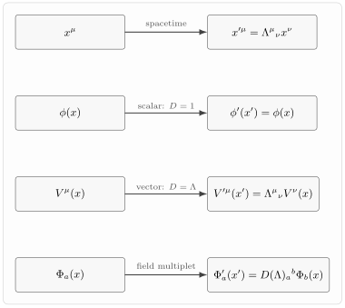
A scalar has no component matrix, while a vector has one Lorentz index. In the passive convention, $x'=\Lambda x$, a scalar obeys $\phi'(x')=\phi(x)$ and a vector obeys $V'^\mu(x')=\Lambda^\mu{}_{\nu}V^\nu(x)$.

The scalar representation and the Klein–Gordon mass shell

The free real scalar field obeys the Klein–Gordon equation

$$(\partial^2+m^2)\phi(x)=0, \qquad \partial^2=\partial_\mu\partial^\mu.$$

Substitute a plane wave

$$\phi(x)=e^{-ip\cdot x}.$$

Since

$$\partial_\mu e^{-ip\cdot x}=-ip_\mu e^{-ip\cdot x},$$

we get

$$\partial^2 e^{-ip\cdot x}=-p^2 e^{-ip\cdot x}.$$

Therefore the equation of motion becomes

$$(-p^2+m^2)e^{-ip\cdot x}=0,$$

or

$$p^2=m^2.$$

This is the mass shell. In components,

$$(p^0)^2-\mathbf p^2=m^2,$$

so the two energy branches are

$$p^0=\pm E_{\mathbf p}, \qquad E_{\mathbf p}=\sqrt{\mathbf p^2+m^2}.$$

In the quantum field, both branches are present in a way compatible with positive energy quanta: the negative-frequency term is the creation part of the field. With the covariant normalization used throughout the relativistic part of the course,

$$\phi(x)=\int {d^3\mathbf p\over (2\pi)^3 2E_{\mathbf p}} \left(a(\mathbf p)e^{-ip\cdot x}+a^\dagger(\mathbf p)e^{ip\cdot x}\right), \qquad p^0=E_{\mathbf p},$$

with

$$[a(\mathbf p),a^\dagger(\mathbf q)] =(2\pi)^3 2E_{\mathbf p}\delta^{(3)}(\mathbf p-\mathbf q).$$

Many canonical calculations instead absorb the $2E_{\mathbf p}$ into the operators and write $d^3p/[(2\pi)^3\sqrt{2E_{\mathbf p}}]$. That convention is equivalent, but the covariant version makes the Lorentz-invariant on-shell measure visible.

The Lorentz representation of the field is trivial, but the momentum labels move along the mass shell. The spin is not hidden in the scalar field; it is absent. The one-particle states created by $a^\dagger(\mathbf p)$ form a spin-zero representation.

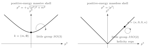
The positive-energy branches are shown in a $p^0$–$p^3$ slice. A massive particle has a rest frame $k^\mu=(m,0,0,0)$ and little group $SO(3)$. A massless particle has no rest frame; a standard momentum is $q^\mu=(\kappa,0,0,\kappa)$, whose little group is the Euclidean group $ISO(2)$ acting in the transverse plane.

One-particle states and little groups

A field representation tells us how local operators transform. Particle spin is more directly classified by one-particle states.

Use relativistically normalized positive-energy one-particle states

$$\langle \mathbf p',\sigma'|\mathbf p,\sigma\rangle =(2\pi)^3 2E_{\mathbf p}\delta^{(3)}(\mathbf p'-\mathbf p)\delta_{\sigma'\sigma}.$$

The associated invariant on-shell measure is

$$\int d\Pi_p=\int {d^3\mathbf p\over(2\pi)^3 2E_{\mathbf p}}.$$

A one-particle state is labeled by a four-momentum on a mass shell and by a discrete label $\sigma$ describing spin or helicity. Under a Lorentz transformation,

$$U(\Lambda)|p,\sigma\rangle =\sum_{\sigma'} C_{\sigma'\sigma}(\Lambda,p)|\Lambda p,\sigma'\rangle.$$

The nontrivial part is not the fact that $p$ becomes $\Lambda p$. The nontrivial part is the matrix $C_{\sigma'\sigma}(\Lambda,p)$ acting on the spin labels.

To understand it, choose a standard momentum $k$ on the mass shell and a standard Lorentz transformation $L(p)$ such that

$$p=L(p)k.$$

For a general Lorentz transformation $\Lambda$, define

$$W(\Lambda,p)=L(\Lambda p)^{-1}\Lambda L(p).$$

This transformation leaves $k$ fixed:

$$W(\Lambda,p)k=k.$$

The set of transformations leaving $k$ fixed is called the little group of $k$. Particle spin labels transform under representations of this little group.

For a massive particle, choose

$$k^\mu=(m,0,0,0).$$

A Lorentz transformation preserving this vector cannot mix time with space. It must act as a spatial rotation. Therefore the massive little group is

$$SO(3),$$

or more precisely its double cover $SU(2)$ for spinor representations. Massive particles are classified by ordinary spin

$$s=0,{1\over2},1,{3\over2},\ldots,$$

with $2s+1$ spin states.

For a massless particle, choose a standard momentum along the $z$-axis,

$$q^\mu=(\kappa,0,0,\kappa), \qquad q^2=0.$$

There is no rest frame. The little group preserving $q$ is not $SO(3)$ but

$$ISO(2),$$

the group of rotations and translations in a two-dimensional Euclidean plane. For the finite-helicity particle representations normally used in local relativistic QFT, the translation-like part acts trivially on physical one-particle states, leaving only rotations around the direction of motion. In gauge-field realizations the same translation-like little-group action is closely related to gauge transformations of polarization vectors. Massless particles are therefore labeled by helicity,

$$h={\mathbf J\cdot \mathbf p\over |\mathbf p|}.$$

A massless scalar has $h=0$. A photon has $h=+1$ and $h=-1$.

This is the first place where a crucial warning appears: field components and particle polarizations are not the same thing. A four-vector field has four components, but a massive spin-one particle has three physical polarizations, while a massless spin-one particle has two.

A practical way to remember the distinction is this: components are counted before imposing equations of motion, constraints, and gauge equivalences; physical polarizations are counted after all of them have been imposed.

Massive vector fields and spin one

A Lorentz vector field $A^\mu(x)$ transforms as

$$A'^\mu(x')=\Lambda^\mu{}_{\nu}A^\nu(x).$$

If $A^\mu$ were just four unrelated scalar fields packaged with a Lorentz index, it would contain too many degrees of freedom for a spin-one particle. A massive spin-one field is instead described by the Proca Lagrangian

$$\mathcal L_{\mathrm{Proca}} =-{1\over4}F_{\mu\nu}F^{\mu\nu} +{1\over2}M^2 A_\mu A^\mu, \qquad F_{\mu\nu}=\partial_\mu A_\nu-\partial_\nu A_\mu.$$

The Euler–Lagrange equation is

$$\partial_\mu F^{\mu\nu}+M^2 A^\nu=0.$$

Taking $\partial_\nu$ of both sides gives

$$M^2\partial_\nu A^\nu=0,$$

because $\partial_\nu\partial_\mu F^{\mu\nu}=0$ by antisymmetry. For $M\neq0$,

$$\partial_\mu A^\mu=0.$$

Then the equation of motion reduces to

$$(\partial^2+M^2)A^\nu=0.$$

For a plane wave

$$A^\mu(x)=\epsilon^\mu(p)e^{-ip\cdot x},$$

we obtain

$$p^2=M^2, \qquad p_\mu\epsilon^\mu(p)=0.$$

The first condition says that the vector mode is on the massive mass shell. The second says that the polarization vector is transverse to the four-momentum. Four components minus one constraint leaves three physical polarizations, exactly the number of spin-one states for a massive particle.

In the rest frame $p^\mu=(M,0,0,0)$, the transversality condition becomes

$$M\epsilon^0=0,$$

so

$$\epsilon^0=0.$$

The three independent polarizations can be chosen as

$$\epsilon_1^\mu=(0,1,0,0), \qquad \epsilon_2^\mu=(0,0,1,0), \qquad \epsilon_3^\mu=(0,0,0,1).$$

They rotate as an ordinary three-vector under the massive little group $SO(3)$. This is why a massive vector field describes spin one, not four independent scalar particles.

With normalization

$$\epsilon_\lambda(p)\cdot \epsilon_{\lambda'}(p)=-\delta_{\lambda\lambda'},$$

the physical polarization sum is

$$\sum_{\lambda=1}^{3} \epsilon_\lambda^\mu(p)\epsilon_\lambda^{*\nu}(p) =-\eta^{\mu\nu}+{p^\mu p^\nu\over M^2}.$$

The right-hand side is the Lorentz-covariant projector onto the subspace orthogonal to $p^\mu$.

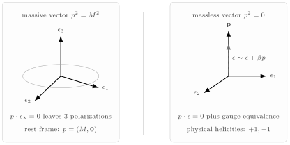
A massive vector has three physical polarizations because $p\cdot\epsilon=0$ leaves a three-dimensional subspace. A massless vector has a gauge equivalence $\epsilon^\mu\sim\epsilon^\mu+\alpha p^\mu$, so only two transverse helicities remain.

Massless vectors and gauge redundancy

The massless vector field is subtler. The Maxwell Lagrangian is

$$\mathcal L_{\mathrm{Maxwell}} =-{1\over4}F_{\mu\nu}F^{\mu\nu}.$$

It is invariant under the gauge transformation

$$A_\mu(x)\longmapsto A_\mu(x)+\partial_\mu\alpha(x).$$

The equations of motion in the absence of sources are

$$\partial_\mu F^{\mu\nu}=0.$$

For a plane wave $A^\mu=\epsilon^\mu e^{-ip\cdot x}$, these become

$$p^2\epsilon^\nu-p^\nu(p\cdot\epsilon)=0.$$

Gauge transformations act on the polarization vector by adding a multiple of the null momentum. With the plane-wave convention $e^{-ip\cdot x}$, the exact sign and factor of $i$ depend on how the gauge parameter is normalized, but the physical equivalence relation is unambiguous:

$$\epsilon^\mu\sim \epsilon^\mu+\beta p^\mu.$$

For a massless on-shell mode, $p^2=0$. One may impose the transverse condition

$$p\cdot\epsilon=0,$$

but this condition alone leaves three independent components: four components minus one constraint. Gauge equivalence removes one more component. Thus the massless vector has

$$4-1-1=2$$

physical polarizations.

Take $p^\mu=(E,0,0,E)$. A convenient pair of transverse polarization vectors is

$$\epsilon_1^\mu=(0,1,0,0), \qquad \epsilon_2^\mu=(0,0,1,0).$$

The circular combinations

$$\epsilon_\pm^\mu={1\over\sqrt2}(0,1,\pm i,0)$$

carry helicity $\pm1$. More explicitly, for an active rotation represented by

$$D(R_z(\theta))=e^{-i\theta J_z},$$

the transverse components obey

$$D(R_z(\theta))\epsilon_+ =e^{-i\theta}\epsilon_+, \qquad D(R_z(\theta))\epsilon_- =e^{+i\theta}\epsilon_-.$$

Thus $J_z\epsilon_\pm=\pm\epsilon_\pm$ for momentum along $+z$. These are the two physical photon polarizations. A passive rotation uses the inverse matrix and therefore reverses the displayed phases, without changing the helicity labels.

The missing longitudinal and timelike components are not missing by accident. They are removed because a massless vector representation with a local Lorentz-covariant field requires gauge redundancy. This fact becomes central when we turn to Maxwell theory, QED, Ward identities, and gauge fixing.

Light-cone coordinates and boost weights

A very efficient way to see boost weights is to temporarily restrict to one time and one space coordinate. Define

$$p_+=p^0+p^1, \qquad p_-=p^0-p^1.$$

Then

$$p^2=(p^0)^2-(p^1)^2=p_+p_-.$$

The scalar mass shell becomes

$$p_+p_-=m^2.$$

A boost of rapidity $\chi$ acts as

$$p'^0=p^0\cosh\chi+p^1\sinh\chi,$$ $$p'^1=p^1\cosh\chi+p^0\sinh\chi.$$

Therefore

$$p'_+=e^{\chi}p_+, \qquad p'_-=e^{-\chi}p_-.$$

The invariant product is unchanged:

$$p'_+p'_-=p_+p_-.$$

Vector components behave the same way. Define

$$V_+=V^0+V^1, \qquad V_-=V^0-V^1.$$

Then

$$V'_+=e^{\chi}V_+, \qquad V'_-=e^{-\chi}V_-.$$

This is a simple way to see the representation content of vectors under boosts: light-cone components are eigenvectors of the boost generator.

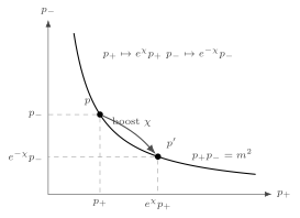
In $1+1$ dimensions, the mass shell is $p_+p_-=m^2$. A boost of rapidity $\chi$ rescales the two light-cone components oppositely: $p_+\mapsto e^{\chi}p_+$ and $p_-\mapsto e^{-\chi}p_-$.

The same light-cone idea previews spinors. Suppose we introduce two components $\psi_+$ and $\psi_-$ with boost weights

$$\psi_+\longmapsto e^{\chi/2}\psi_+, \qquad \psi_-\longmapsto e^{-\chi/2}\psi_-.$$

Then the pair of first-order equations

$$p_-\psi_+=m\psi_-, \qquad p_+\psi_-=m\psi_+$$

is boost covariant. Indeed, under a boost,

$$p_-\psi_+\longmapsto e^{-\chi}p_-\,e^{\chi/2}\psi_+ =e^{-\chi/2}p_-\psi_+,$$

which transforms like $\psi_-$. Similarly, $p_+\psi_-$ transforms like $\psi_+$.

Combining the two first-order equations gives

$$p_+p_-\psi_+=m^2\psi_+, \qquad p_+p_-\psi_-=m^2\psi_-.$$

Thus each component satisfies the scalar mass-shell equation, but the two-component object carries a nontrivial boost representation. This is the simplest algebraic shadow of the Dirac equation: a relativistic first-order equation can be viewed as a square root of the scalar mass-shell condition.

In the massless case, the equations decouple:

$$p_-\psi_+=0, \qquad p_+\psi_-=0.$$

The two components propagate on opposite light-cone branches. This is the two-dimensional ancestor of chirality.

Field representations versus particle representations

It is tempting to say “a scalar field is spin zero” and “a vector field is spin one.” These statements are useful shortcuts, but the precise relationship is more structured.

A field representation is finite-dimensional. For example, the four-vector representation is four-dimensional. However, the Lorentz group is noncompact, so its nontrivial finite-dimensional representations are not unitary. Particle states, on the other hand, live in a Hilbert space and transform unitarily. The little group reconciles these statements: one-particle spin labels transform under compact little groups for massive particles, and under helicity representations for massless particles.

This is why “a vector field has four components” is not a particle-counting statement. The local field is deliberately redundant enough to transform simply under Lorentz transformations. The physical Hilbert-space degrees of freedom emerge only after the mass shell, constraints, and possible gauge equivalences are taken into account.

For a massive vector field, the Proca constraint $p\cdot\epsilon=0$ selects the three-dimensional subspace that transforms as spin one in the rest frame. For a massless vector field, gauge redundancy further identifies polarizations differing by $p^\mu$, leaving two helicities.

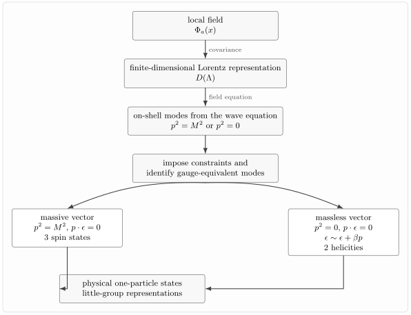
A local field carries a finite-dimensional Lorentz representation. On the mass shell, equations of motion, constraints, and gauge equivalences reduce field components to physical particle labels: spin states for massive particles and helicities for massless particles.

This distinction becomes especially important for spinor fields. A Weyl spinor is a finite-dimensional Lorentz representation, while a physical massless spinor particle is labeled by helicity. The next pages develop this in detail using gamma matrices and the Dirac equation.

Summary

A scalar field transforms trivially under Lorentz transformations, but its plane-wave modes still move on Lorentz-invariant mass shells. The Klein–Gordon equation imposes

$$p^2=m^2,$$

and the scalar field creates spin-zero one-particle states.

A vector field transforms with a Lorentz matrix. A massive vector field is not just four scalar fields: the Proca equation implies the transversality condition

$$p\cdot\epsilon=0,$$

leaving three physical polarizations, as required for a massive spin-one particle. A massless vector field has gauge redundancy

$$\epsilon^\mu\sim \epsilon^\mu+\beta p^\mu,$$

which leaves only two transverse helicities.

The particle classification comes from little groups. Massive particles have little group $SO(3)$ and are labeled by spin. Massless particles have little group $ISO(2)$, and the ordinary local particle representations are labeled by helicity. Field representations and particle representations are related, but they are not identical.

Light-cone coordinates make boost weights transparent. In $1+1$ dimensions,

$$p_+\to e^\chi p_+, \qquad p_-\to e^{-\chi}p_-,$$

so the mass shell $p_+p_-=m^2$ is manifestly invariant. The same idea previews spinors, whose components transform with half-boost weights.

Common pitfalls

• A scalar field is not invariant as a function of the same coordinate values. The correct statement is $\phi'(x')=\phi(x)$ for the same physical event. Equivalently, $\phi'(x)=\phi(\Lambda^{-1}x)$.
• A four-vector field does not automatically describe four physical particles. The physical degrees of freedom are determined after imposing equations of motion, constraints, and possible gauge equivalences.
• Count physical polarizations only after imposing all restrictions. The condition $p\cdot\epsilon=0$ removes one component, not two. For a massless vector, the second removal comes from gauge equivalence $\epsilon\sim\epsilon+\beta p$.
• Do not confuse field representation labels with particle spin labels. A Lorentz field may contain several rotational spins before constraints are imposed. For example, the four-vector representation decomposes under spatial rotations into a time component and a spatial vector.
• Massless particles do not have rest frames. Their spin is not classified by rest-frame $SO(3)$ but by helicity.
• Do not mix covariant creation operators with the $1/\sqrt{2E_{\mathbf p}}$ oscillator convention inside the same calculation. The two descriptions are equivalent only after rescaling the operators and states; otherwise LSZ factors and polarization sums acquire spurious powers of $2E_{\mathbf p}$.

Exercises

Exercise 1: scalar covariance of the Klein–Gordon equation

Show that the Klein–Gordon equation is Lorentz covariant for a scalar field. Use

$$\phi'(x')=\phi(x), \qquad x'=\Lambda x,$$

and

$$\Lambda^T\eta\Lambda=\eta.$$

Solution

The derivative with respect to the transformed coordinate is

$$\partial'_\mu={\partial x^\nu\over \partial x'^\mu}\partial_\nu =(\Lambda^{-1})^\nu{}_\mu\partial_\nu.$$

Raising the index gives

$$\partial'^\mu=\eta^{\mu\rho}\partial'_\rho.$$

The d’Alembertian is

$$\partial'^2=\partial'_\mu\partial'^\mu =\eta^{\mu\rho}(\Lambda^{-1})^\nu{}_\mu(\Lambda^{-1})^\sigma{}_\rho \partial_\nu\partial_\sigma.$$

Lorentz invariance of the metric implies

$$\eta^{\mu\rho}(\Lambda^{-1})^\nu{}_\mu(\Lambda^{-1})^\sigma{}_\rho =\eta^{\nu\sigma}.$$

Therefore

$$\partial'^2=\eta^{\nu\sigma}\partial_\nu\partial_\sigma=\partial^2.$$

Since $\phi'(x')=\phi(x)$,

$$(\partial'^2+m^2)\phi'(x')=(\partial^2+m^2)\phi(x).$$

Thus if $\phi$ solves the Klein–Gordon equation, so does $\phi'$.

Exercise 2: the massive-vector polarization projector

For a massive vector particle, define

$$\Pi^{\mu\nu}(p)=-\eta^{\mu\nu}+{p^\mu p^\nu\over M^2}, \qquad p^2=M^2.$$

Show that $p_\mu\Pi^{\mu\nu}=0$ and that $\eta_{\mu\nu}\Pi^{\mu\nu}=-3$.

Solution

First contract with $p_\mu$:

$$p_\mu\Pi^{\mu\nu} =-p_\mu\eta^{\mu\nu}+{p_\mu p^\mu p^\nu\over M^2}.$$

Since $p_\mu\eta^{\mu\nu}=p^\nu$ and $p_\mu p^\mu=p^2=M^2$,

$$p_\mu\Pi^{\mu\nu} =-p^\nu+{M^2p^\nu\over M^2}=0.$$

Now take the trace:

$$\eta_{\mu\nu}\Pi^{\mu\nu} =-\eta_{\mu\nu}\eta^{\mu\nu}+{\eta_{\mu\nu}p^\mu p^\nu\over M^2}.$$

In four spacetime dimensions,

$$\eta_{\mu\nu}\eta^{\mu\nu}=4,$$

and

$$\eta_{\mu\nu}p^\mu p^\nu=p^2=M^2.$$

Therefore

$$\eta_{\mu\nu}\Pi^{\mu\nu}=-4+1=-3.$$

The minus sign reflects the mostly-minus metric and the convention $\epsilon_\lambda\cdot\epsilon_\lambda=-1$ for physical massive vector polarizations. The number of physical polarizations is $3$.

Exercise 3: covariance of the light-cone equations

Let

$$p_+=p^0+p^1, \qquad p_-=p^0-p^1.$$

A boost of rapidity $\chi$ gives $p_+\to e^\chi p_+$ and $p_-\to e^{-\chi}p_-$. Suppose

$$\psi_+\to e^{\chi/2}\psi_+, \qquad \psi_-\to e^{-\chi/2}\psi_-.$$

Show that the equations

$$p_-\psi_+=m\psi_-, \qquad p_+\psi_-=m\psi_+$$

are boost covariant.

Solution

Under the boost,

$$p_-\psi_+\to (e^{-\chi}p_-)(e^{\chi/2}\psi_+) =e^{-\chi/2}p_-\psi_+.$$

The right-hand side transforms as

$$m\psi_-\to m e^{-\chi/2}\psi_-.$$

Thus the first equation transforms with the same overall factor on both sides.

Similarly,

$$p_+\psi_-\to (e^\chi p_+)(e^{-\chi/2}\psi_-) =e^{\chi/2}p_+\psi_-,$$

while

$$m\psi_+\to m e^{\chi/2}\psi_+.$$

The second equation is also covariant. The half-boost weights are precisely what make a first-order square root of the mass shell compatible with Lorentz boosts.

Exercise 4: transverse polarizations and helicity

Consider a massless vector with standard momentum

$$p^\mu=(E,0,0,E).$$

Show that the transverse polarization vectors

$$\epsilon_\pm^\mu={1\over\sqrt2}(0,1,\pm i,0)$$

satisfy $p\cdot\epsilon_\pm=0$. Then use

$$D(R_z(\theta))=e^{-i\theta J_z}$$

to determine their rotation phases and helicities.

Solution

The scalar product is

$$p\cdot\epsilon_\pm =p^0\epsilon_\pm^0-p^1\epsilon_\pm^1-p^2\epsilon_\pm^2-p^3\epsilon_\pm^3.$$

For $p^\mu=(E,0,0,E)$ and $\epsilon_\pm^\mu=(0,1,\pm i,0)/\sqrt2$,

$$p\cdot\epsilon_\pm=E\cdot0-0-0-E\cdot0=0.$$

For an active rotation by angle $\theta$ around the $z$-axis, the transverse components transform as

$$\begin{pmatrix} \epsilon'^1\\ \epsilon'^2 \end{pmatrix} = \begin{pmatrix} \cos\theta&-\sin\theta\\ \sin\theta&\cos\theta \end{pmatrix} \begin{pmatrix} \epsilon^1\\ \epsilon^2 \end{pmatrix}.$$

Applying this matrix to the two circular polarization vectors gives

$$D(R_z(\theta))\epsilon_+ =e^{-i\theta}\epsilon_+, \qquad D(R_z(\theta))\epsilon_- =e^{+i\theta}\epsilon_-.$$

Because $D(R_z(\theta))=e^{-i\theta J_z}$, it follows that

$$J_z\epsilon_+=+\epsilon_+, \qquad J_z\epsilon_-=-\epsilon_-.$$

The momentum points along $+z$, so $h=J_z$. Therefore $\epsilon_+$ has helicity $+1$ and $\epsilon_-$ has helicity $-1$. The opposite phases would appear in a passive rotation, which uses the inverse rotation matrix.

Further reading

• Sidney Coleman, Lectures on Quantum Field Theory, edited by Bryan Gin-ge Chen et al., World Scientific, 2019, chapters 18 and 26.
• Mark Srednicki, Quantum Field Theory, Cambridge University Press, 2007, sections 33, 34, and 54–56.
• Steven Weinberg, The Quantum Theory of Fields, Volume I: Foundations, Cambridge University Press, 1995, sections 2.5 and 5.3.
• A. Zee, Quantum Field Theory in a Nutshell, 2nd edition, Princeton University Press, 2010, chapter II.3.

References

Section titled “References”- Schwartz, Matthew D. Quantum Field Theory and the Standard Model. Cambridge University Press, 2014. DOI.