

Fermi Surface and Nonrelativistic Many-Body Fields
The previous pages treated current correlators as response functions in relativistic field theory. We now put a quantum field theory in a medium. The cleanest medium is a zero-temperature nonrelativistic Fermi gas. Its ground state is not empty space; it is a filled Fermi sea. This single change reorganizes perturbation theory: the propagator knows whether a momentum state is occupied, low-energy excitations live near a surface in momentum space, and density response is controlled by particle-hole pairs rather than by particle-antiparticle pairs.
The central object is therefore not a fluctuation near , but a fluctuation near
A Fermi liquid has gapless modes at every point of a codimension-one surface. This is why many-body field theory feels familiar to a quantum field theorist but not identical to relativistic QFT: locality in spacetime remains, yet scaling is organized around a surface rather than around an isolated point.
This page develops the free nonrelativistic fermion field, derives the finite-density propagator and its pole prescription, linearizes the theory near the Fermi surface, and computes the first density-response formula. The next page uses the same tools to study one-dimensional singularities and Fermi-surface instabilities.
Required background. Current correlators and polarization tensors supplies the response-function and contour logic used for the density bubble. Helpful background. Contact scattering and renormalization in quantum mechanics supplies the nonrelativistic normalization used below.
A useful way to read the page is to keep three energies separate:
Low energy means small , not small and not small .
One organizing principle to keep in mind is that finite density changes the scaling problem. Near a Fermi surface, normal momentum and frequency scale to zero, while tangential momentum mostly labels the patch. This is why four-fermion interactions that would look irrelevant by relativistic power counting can become marginal in Fermi-surface kinematics.
The nonrelativistic field at finite density
Section titled “The nonrelativistic field at finite density”Finite-density conventions. We use real time and set . The free grand-canonical Hamiltonian is
so the free action is
In momentum space,
At zero temperature,
The time-ordered Green function is defined by
where is the filled Fermi sea.
A spinless nonrelativistic fermion field satisfies
The particle number is
and a general two-body interaction can be written as
For the free theory, the dispersion measured relative to the chemical potential is
The ground state at fills all one-particle modes with . Thus
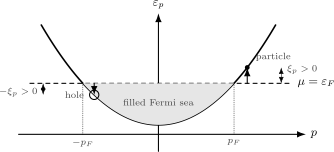
The nonrelativistic ground state at finite density fills all states below the Fermi energy. A low-energy particle lies just outside the Fermi surface, while a low-energy hole is a missing occupied state just inside it.
The unindexed field and single-particle formulas describe one species. For independent internal states, such as two spin states with no splitting, restore an index and sum their Hamiltonians and number operators. We assume all species have the same , and , so
Hereafter , , and denote totals over these species. The density is
where
is the area of the unit -sphere. The density of states at the Fermi surface is
This number is also the zero-temperature density susceptibility, often called the compressibility in many-body notation,
The mechanical isothermal compressibility includes an additional factor of the density,
We use on this page because that is the quantity that enters density response and Thomas–Fermi screening.
The formula is simple but conceptually important. At low energy, most states in the filled sea are inert. Response comes from a thin shell near , and the size of that shell is measured by the density of states on the surface.
Particle and hole excitations
Section titled “Particle and hole excitations”Let annihilate a fermion in the momentum mode . The Fermi-sea occupation rule is
while
For , the operator creates a particle excitation with energy . For , the operator removes an occupied fermion and creates a hole excitation with energy
A finite-density fermion problem is therefore naturally a particle-hole theory. In a relativistic vacuum, all positive-energy particle modes are empty. In a Fermi sea, the sign of decides whether the elementary excitation is created by or by .
For a density perturbation carrying momentum ,
the operator removes a fermion from and puts it at . It contributes to low-energy response only when
or through the reverse process at negative frequency. For , this restricts to a narrow strip of width around the Fermi surface.
The energy of such a particle-hole pair is
Near the Fermi surface, with ,
At leading order in , the response is controlled by the angle between the momentum transfer and the local Fermi-surface normal.
The finite-density propagator
Section titled “The finite-density propagator”The field evolves as
For ,
For , time ordering interchanges the fermion operators and gives an additional minus sign, so
Thus
Fourier transforming with
gives
Equivalently,
This compact formula contains the essential finite-density pole prescription. If , the state is empty and the pole is below the real axis, just like a particle propagating forward in time. If , the state is occupied and the pole is above the real axis, corresponding to a hole propagating backward in the time-ordered function.
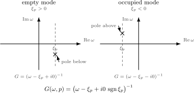
The time-ordered propagator knows which modes are occupied. Empty modes have the usual particle pole below the real axis, while occupied modes have the pole above the real axis. The Fermi surface is where this prescription changes.
The retarded Green function has a different prescription:
It puts all poles below the real axis, independent of occupation, because it is fixed by causal response rather than by ground-state time ordering. The occupation information then enters response functions through the state, not through moving retarded poles above the axis. Mixing these two propagators is one of the most common sources of wrong signs in many-body calculations.
A good rule of thumb is: use the time-ordered propagator for ground-state perturbation theory and diagrammatic expansions of expectation values; use the retarded propagator for causal response. The two are related by spectral functions and occupation factors, but they are not interchangeable inside loop integrals.
Linearizing near the Fermi surface
Section titled “Linearizing near the Fermi surface”For low-energy processes, write
where is a unit vector normal to the Fermi surface and . Split into normal and tangential pieces,
Then
At the lowest energies,
The momentum-space measure near the surface becomes
up to curvature corrections. This is why the density of states is a surface quantity. The angular variable labels a patch; the normal momentum controls the low-energy cost.
The tangential momentum labels which nearby point of the Fermi surface the excitation belongs to. It does not cost energy to move along the Fermi surface at leading order. This is the geometric difference between a Fermi surface and an isolated relativistic node.
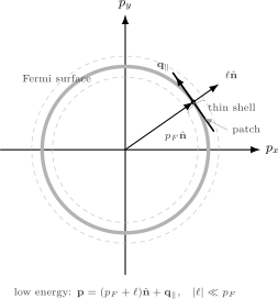
A low-energy mode near a Fermi surface is described by a patch label and a small normal displacement . To leading order, ; tangential momenta label nearby gapless modes.
To write a real-space low-energy theory, cover the Fermi surface by patches labeled by , with normals , and expand
Here varies slowly on the scale . Acting with the free inverse propagator gives
Thus the leading patch action is
Curvature terms such as are subleading for many questions, but they should not be forgotten. They regulate collinear degeneracies and determine the finite size of a patch in a controlled scaling limit. In particular, a patch theory is not obtained by declaring all tangential momenta equally low-energy forever; the patch width is tied to the energy resolution and to the curvature of the original Fermi surface.
The corresponding shell scaling keeps the patch label fixed while sending
This scaling does not make every four-fermion process equally important. Momentum conservation leaves exceptional low-energy channels: forward scattering between nearby patches and Cooper scattering between nearly opposite patches. In one dimension the Fermi surface has only two patches, so the same right- and left-moving fields recur in several exceptional channels. That overlap is the origin of the enhanced logarithms on the next page.
The two Fermi points in one dimension
Section titled “The two Fermi points in one dimension”In one spatial dimension the Fermi surface consists of two points, and . The low-energy expansion becomes especially transparent:
For momenta near the right Fermi point,
For momenta near the left Fermi point,
The leading low-energy action is therefore
The inverse propagators are
for the time-ordered zero-temperature functions, because occupation changes as crosses zero at each Fermi point.
This is the doorway to the next page. In one dimension, right- and left-moving fermions have very restricted kinematics. Particle-hole loops become singular, density waves become strong, and weak interactions can reorganize the ground state.
Density response and the particle-hole bubble
Section titled “Density response and the particle-hole bubble”Couple the same weak external potential energy to every species, through the total density,
In the action this appears with the opposite sign,
The quadratic response is determined by the density-density bubble. The retarded response function is
The free Hamiltonian does not mix species. Density bilinears from distinct species commute, and their connected response vanishes. Consequently,
The subscript means the response of one species. There is one species sum around each bubble, not two independent sums at its density vertices. For the total free-gas response,
This is the Lindhard function. It is the same particle-hole kinematics described above, now packaged as a response kernel. The state sum and retarded boundary condition originate in Lindhard 1954, § 3, pp. 28–29, Eqs. (3.1)–(3.3), PDF. His longitudinal dielectric function is ; here is a number-density response to potential energy, not the electric susceptibility. The explicit spin-degenerate bubble and static density of states are Altland and Simons 2023, § 4.2, pp. 194–195, Eqs. (4.28)–(4.32), with their factor replaced by .
The occupation-number numerator is worth deriving because it makes the allowed processes visible. If
then
Consequently,
The first term excites an occupied state into an empty one and has a positive-frequency pole. The second is the reverse process and supplies the negative-frequency pole. This is the spectral counterpart of the contour statement from the previous page: a loop contributes when the occupation-dependent poles lie on opposite sides of the energy contour.
The diagram follows one species around the loop. Sum the identical loops to obtain the response to the common source.
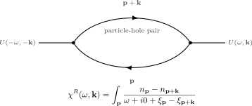
Each unit density insertion preserves the species label while transferring momentum and energy . The displayed single-species response is summed once over identical independent species for a common source. The total density of states uses the same factor. Schematic topology; the retarded response is obtained with the displayed frequency prescription, not by replacing both internal lines with retarded single-particle propagators.
Two limits are worth separating. First, for exactly and nonzero frequency,
A spatially uniform time-dependent source coupled to total particle number cannot change the density of a system with conserved ; it only changes the phase of states with definite particle number.
Second, the static long-wavelength response gives the compressibility. Since enters the single-particle energy as , a positive lowers the density. Thus
Correspondingly,
for the convention . If instead one couples a source as a local chemical-potential shift, then and the response is .
The two small- limits do not commute:
This noncommutativity is a compact signature of finite density. It is not a paradox; it says that a static source allows particles to rearrange near the Fermi surface, whereas a perfectly uniform time-dependent source cannot create particle-hole pairs. Operationally, the static limit measures equilibrium thermodynamics, while the uniform dynamic limit measures a conservation law.
Static screening as a first application
Section titled “Static screening as a first application”Suppose all species interact through the same density-density potential . In the static, long-wavelength Thomas–Fermi approximation, use the total free-gas susceptibility as the irreducible density response. A test potential is dressed by the induced total density, giving
With the present sign convention, the self-consistency equations are
Eliminating gives the displayed denominator. The plus sign is therefore physical rather than decorative: repulsive density fluctuations oppose the applied potential energy.
For three-dimensional Coulomb repulsion, specify the potential-energy strength by . With a canonically normalized Maxwell field, a charge of magnitude has Gauss flux and hence potential . Its pair potential therefore has
Here is the charge in Gaussian electrostatic units. Thus the frequently used many-body expression does not insert an extra into the canonically normalized QED charge. Equivalently, fixes the Fourier transform. We take an inert uniform neutralizing background, remove the uniform Coulomb component, and consider . No background dielectric constant is included; if one is prescribed, replace by .
Substituting this interaction gives
This is the screening length of Altland and Simons 2023, § 4.2, pp. 197–198, Eqs. (4.39)–(4.40): their equals , and their includes both spin states. The use of the free bubble inside the self-consistent potential neglects exchange and vertex corrections; it does not identify the full interacting compressibility with . Coulomb Screening, Dielectric Response, and RPA explains the approximation and its range.
The Fermi surface screens long-range electric fields. The same algebra with an attractive interaction has the opposite sign in the denominator; if the denominator vanishes at small , the homogeneous state is unstable. This is the many-body field-theory version of the familiar distinction between electric screening and gravitational Jeans instability.
Within this static approximation, a vanishing denominator signals loss of stability of the assumed homogeneous state. A pole at a nonzero real frequency can instead describe a stable collective oscillation; the static instability criterion is not a rule for every dynamical pole.
Example: compressibility in two and three dimensions
Section titled “Example: compressibility in two and three dimensions”For spin degeneracy , the density of states at the Fermi level is
In two dimensions, , so
It is independent of . This is a special feature of the parabolic dispersion in two dimensions.
In three dimensions, , so
Thus a three-dimensional Fermi gas becomes more compressible as the Fermi momentum increases. In both cases, the low-energy response is a surface property: the formulas count states in a thin shell around , not all states in the filled sea.
Summary
Section titled “Summary”A nonrelativistic Fermi gas at zero temperature is expanded around a filled Fermi sea, not an empty vacuum. The single-particle energy relevant for low-energy physics is
and the Fermi surface is the locus . Particles live just outside the surface; holes live just inside it.
The finite-density time-ordered propagator is
so the pole prescription changes across the Fermi surface. Low-energy modes are described patch by patch, with
where is the momentum normal to the surface. Density perturbations create particle-hole pairs, and their one-loop response is the Lindhard function
The static limit measures compressibility; the dynamic uniform limit is constrained by particle-number conservation. This is the kinematic foundation for Fermi-liquid theory, screening, and the one-dimensional instabilities that appear next.
Common pitfalls
Section titled “Common pitfalls”Treating the chemical potential as a small insertion. It changes the ground state. Expanding around the empty vacuum and adding later misses the Fermi sea.
Using the retarded prescription inside the time-ordered propagator. Time ordering knows whether a mode is occupied; retarded response only knows causality.
Equating low energy with small momentum. Low energy means small , so momenta lie near , not near the origin.
Interchanging the static and uniform limits. The limits and of the density response need not commute. Compressibility is a static limit; number conservation controls the uniform dynamic limit.
Confusing potential energy with chemical potential. A scalar potential energy and a chemical-potential shift have opposite signs in the Hamiltonian. The density susceptibility is positive, but the response to a positive potential energy is negative.
Calling the mechanical compressibility without qualification. The quantity used in response theory is ; the isothermal mechanical compressibility is .
Exercises
Section titled “Exercises”Exercise 1: Count states and derive the compressibility
Section titled “Exercise 1: Count states and derive the compressibility”For a spin degeneracy , show that the zero-temperature density of a free nonrelativistic Fermi gas in spatial dimensions is
and that
Solution
The density is the number of occupied momentum states per unit volume:
Using spherical coordinates in momentum space,
so
Because
we find
Exercise 2: Derive the filled-sea pole prescription
Section titled “Exercise 2: Derive the filled-sea pole prescription”Starting from
derive
Solution
Use convergence factors for the two time domains:
and
The part gives
The part gives
Adding the two terms gives the result.
Exercise 3: Linearize about the two Fermi points
Section titled “Exercise 3: Linearize about the two Fermi points”In one dimension, define
Neglect terms oscillating as and keep only terms linear in derivatives. Show that
Solution
The free inverse operator is
For the right-moving component,
The term cancels . Dropping gives
For the left-moving component,
so the leading operator is
The cross terms carry phases and average out for smooth low-energy probes. This gives the stated action.
Exercise 4: Compare the static and uniform response limits
Section titled “Exercise 4: Compare the static and uniform response limits”Use the Lindhard formula
to show that for , and that the static response to a common potential energy is . For two identical species, compare this with a perturbation coupled only to species , keeping their unperturbed chemical potentials fixed.
Solution
For , the numerator is exactly zero:
Therefore
for nonzero .
For the static limit, expand at small :
and
Thus
At ,
Therefore
Since raises the single-particle energy, . A chemical-potential shift has the opposite sign, giving .
For a source only on species , the free response matrix is diagonal. Thus , , and . A common source acts on both species and doubles this response. For unequal dispersions or chemical potentials, sum the distinct single-species responses instead of multiplying one of them by .
Exercise 5: Derive Thomas–Fermi screening
Section titled “Exercise 5: Derive Thomas–Fermi screening”For a repulsive Coulomb interaction in the three-dimensional neutralized gas, with ,
and static compressibility , derive the Thomas–Fermi screened potential
Solution
The density responds to a total potential energy as
The induced Hartree potential energy is , so
Solving for gives
Substituting the Coulomb potential gives
Thus
The sign bookkeeping depends on whether one calls an electric potential or the potential energy of an electron. The invariant statement is that repulsive Coulomb interactions reduce the long-wavelength response by the denominator .
References
Section titled “References”- Altland, Alexander, and Ben Simons. Condensed Matter Field Theory. 3rd ed. Cambridge University Press, 2023. DOI.
- Lindhard, Jens. “On the Properties of a Gas of Charged Particles.” Kongelige Danske Videnskabernes Selskab, Matematisk-fysiske Meddelelser 28, no. 8 (1954): 1–57. Open PDF, University of Southern Denmark archive.
Further reading
Section titled “Further reading”- A. L. Fetter and J. D. Walecka, Quantum Theory of Many-Particle Systems (McGraw–Hill, 1971).
- G. D. Mahan, Many-Particle Physics, 3rd ed. (Kluwer Academic/Plenum Publishers, 2000).
- R. Shankar, “Renormalization-group approach to interacting fermions,” Reviews of Modern Physics 66 (1994),129–192. DOI.
- A. Zee, Quantum Field Theory in a Nutshell, 2nd ed. (Princeton University Press, 2010).