

Finite Conformal Maps, Gauge Symmetry, and Free Fields
How does a primary field transform under a finite conformal map? Its local scale and rotation determine a Jacobian factor, but using that factor in a correlator also requires the correct state, domain and, for spinful fields, a compatible choice of frame. This lesson derives the Möbius covariance of separated Euclidean primary correlators and distinguishes a global symmetry from a map between backgrounds.
In dimensions , the connected conformal group is finite-dimensional. In two Euclidean dimensions, however, orientation-preserving local conformal transformations are holomorphic maps. This gives a much larger local symmetry and eventually leads to the Virasoro algebra. The present page is the bridge: first we write the finite transformation law for primary fields, then we separate global Möbius transformations from general local maps, and finally we compare conformal covariance with two other local-symmetry ideas—diffeomorphism invariance and gauge invariance. The page ends by returning to the simplest dynamical fields, free oscillator modes, because the next pages will use their Wightman functions and prescriptions as the basic analytic examples.
Required background. Lesson 15 supplies primary weights, conformal correlators, and the two-dimensional notation used here.
Helpful background. Lesson 14 develops finite conformal transformations and inversion in general dimension, while QFT I, Lesson 37 introduces covariant derivatives, gauge redundancy, and Wilson-line logic.
Primary fields under finite maps
Section titled “Primary fields under finite maps”A holomorphic map rescales lengths locally. Since
the metric transforms as
Thus, to linear order in its radius, a small circle near is mapped to a small circle near , multiplied by the local scale and rotated by the phase of . Nonlinear terms in can distort a finite circle, but that distortion vanishes relative to its radius in the local limit. A primary field responds to the linear scale and rotation with weights .
For a pure dilation and rotation,
the transformation factor is
This is the cleanest way to remember the meanings of and . The sum measures response to local scale, while the difference measures response to local rotation. For a single-valued bosonic local field on the plane, is an integer. Fermions have half-integer spin and require a spin structure; the Ising Majorana fields have weights and .
For noninteger weights, these powers require compatible analytic branches. Choose the frame continuously along the map and insertion configuration, avoiding poles and coincident insertions; do not choose independent principal powers at each point. For half-integer spin this is a choice of lift to the spin frames. A frame rotation then has its appropriate fermionic sign even though it is the identity on coordinates. The Möbius example below makes this qualification concrete.
If the vacuum is invariant under the transformation, correlation functions obey
where
The conformal plane vacuum is invariant under the global generators, with the appropriate cover acting on spinful fields; see Di Francesco, Mathieu and Sénéchal 1997, §6.2.2, p.157, Eq.6.26. The displayed identity assumes that vacuum and uses separated insertions. For a general local map, compare the transported states and domains instead of asserting invariance of the original correlator. The stress tensor is not a primary under arbitrary local maps: it acquires the Schwarzian term studied later.
Global maps and Möbius transformations
Section titled “Global maps and Möbius transformations”The infinitesimal holomorphic transformations are
Locally, can be any holomorphic function. Globally on the Riemann sphere, however, regularity of the vector field at every finite point and at permits only a quadratic polynomial:
These three terms generate translations, dilations plus rotations, and special conformal transformations. Exponentiating them gives the Möbius maps
The matrices
and its negative define the same coordinate map, so the group is on the Riemann sphere. The matrix action on spin frames can distinguish the two lifts. The vector-field derivation is completed in Exercise 2; the finite maps are discussed in Di Francesco, Mathieu and Sénéchal 1997, §§5.1.1–5.1.2, pp.113–114.
The group preserving the upper half-plane is : choose real coefficients and positive determinant, then rescale to . For a real projective matrix before that normalization,
Setwise preservation of the extended real line alone also permits negative determinant. Those transformations exchange the upper and lower half-planes: is an example. The full real-line-preserving group is , with these two components. A common complex rescaling can normalize either component’s determinant, but it cannot make a negative-determinant real representative both real and determinant one.
It is useful to record the elementary identities
and
These identities explain why two-dimensional two-point functions are Möbius covariant. For a primary of weights with a nonzero identical-field pairing,
For complex fields, use the corresponding nonzero paired two-point function. Using the two identities above with the compatible powers just specified,
and similarly for the antiholomorphic part. Thus
For a scalar primary with , this becomes the familiar rotationally invariant form
For a chiral field with , the correlator is holomorphic away from coincident points:
The Ising fermion corresponds to , so its chiral two-point function is proportional to .
For example, take . Although , its spin-frame square root must be chosen as a continuous lift such as . At and , the lifted Jacobian product is , and
Taking both numerical principal square roots to be instead gives and destroys covariance. The missing sign records incompatible frames, not a failure of the fermion two-point function.
Domains, boundaries, and the meaning of covariance
Section titled “Domains, boundaries, and the meaning of covariance”A conformal map may act in two related but conceptually different ways. It may be an automorphism of the same background, such as a Möbius transformation of the plane vacuum. Or it may map one domain to another domain. In the second case, the correlator in the original domain is related to a correlator in the image domain by local Jacobian factors:
Here is a conformal bijection between the domains, the brackets denote normalized correlators, and the boundary condition, state and spin structure are carried from to . An unnormalized partition function can additionally contain Weyl-anomaly factors. A concrete example is the upper-half-plane-to-strip map with corresponding boundary conditions in Di Francesco, Mathieu and Sénéchal 1997, §11.2.3, pp.419–420.
This distinction between a change of description and a symmetry also appears for general coordinate maps. A scalar’s active pullback is
so a coordinate-labeled correlator transforms covariantly:
In an ordinary QFT on a fixed background, this is a useful symmetry statement when preserves the relevant background structure. In a gravitational theory, local diffeomorphisms treated as gauge redundancies, such as transformations supported away from a boundary, make a coordinate-labeled local field insufficient by itself as a physical observable. Physical observables must be invariant under that redundancy or relationally dressed. Transformations acting nontrivially at a physical or asymptotic boundary can instead carry charges and require a separate analysis.
The group is therefore relevant to an upper-half-plane background, provided its boundary condition is also preserved. A map that exchanges the half-planes, or changes the boundary state, is not a symmetry of that specified problem. The need to preserve both the geometric boundary and its condition is emphasized in Di Francesco, Mathieu and Sénéchal 1997, §11.2.1, pp.413–414.
Gauge symmetry and dressed correlators
Section titled “Gauge symmetry and dressed correlators”The same warning appears in gauge theory in a simpler, more familiar form. Consider a charged scalar field in Abelian gauge theory, with convention
The local field is charged. Therefore the naive two-point function
is not a gauge-invariant observable: its phase changes by
There are two standard cures. The first is to make a local neutral composite, such as
The second is to dress the separated charged fields by a Wilson line along a path from to :
This is the inverse of the site-wide forward transporter along the same oriented path:
where and has the opposite orientation. The reversed sign is therefore a path-orientation map, not a different covariant-derivative convention.
Since
the bilocal operator
is gauge invariant. In the figure, follow the three phase factors from the left endpoint to the right: the line cancels the two endpoint transformations. Different paths generally define different dressed operators. In a continuum quantum theory, the local neutral product and the line-dressed bilocal also require their appropriate composite-operator and line renormalization; gauge invariance alone does not establish finiteness.
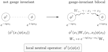
A separated charged pair acquires two independent endpoint phases. Along the chosen path , supplies their inverse product, making the dressed bilocal gauge invariant. The path is schematic; it is not a propagator or a claim of path independence.
This is the gauge-theory analogue of the gravity warning above. Local charged fields are perfectly useful inside a fixed gauge or as ingredients in correlation functions, but physical questions must be expressed in gauge-invariant terms. In later pages Wilson loops will become central order parameters for confinement.
Free fields as oscillator modes
Section titled “Free fields as oscillator modes”We now return to a simpler system: the free scalar field. The reason is strategic. The next page studies Wightman functions, commutators, and the prescription. All of those analytic structures can be seen already in the free oscillator decomposition.
Let a real free scalar of mass live in -dimensional Minkowski spacetime, with spatial momentum components. The positive mass makes every mode below a genuine oscillator. With periodic boundary conditions in a finite spatial volume , write
with
The creation and annihilation operators obey
The time-dependent oscillator mode is normalized by its Wronskian:
Indeed, for ,
This Wronskian is the mode-by-mode version of the canonical commutation relation
Indeed, inserting the mode expansion, relabeling in the second term, and using gives
where is the periodic delta function. This displays directly why the sign and normalization of the Wronskian matter. If in a periodic box, the spatially constant mode has and cannot use . Its canonical variables and have the free-particle Hamiltonian and must be quantized separately. The two-dimensional massless example is worked out in Di Francesco, Mathieu and Sénéchal 1997, §6.3.1, pp.159–160; after rescaling its scalar to a canonical kinetic term, it has this same zero-mode structure.
In infinite volume,
and the expansion becomes
The continuum operators are rescaled relative to their box counterparts, before the limit. Suppressing those labels in the continuum expansion gives
In this limit becomes the ordinary spatial delta distribution. For Euclidean momentum , define . The infinite-volume vacuum covariance is
where is the Euclidean norm squared. It is the coefficient after removing the momentum delta, not the full coincident-momentum expectation, that equals the inverse kernel. Applying to the corresponding position-space covariance gives .
At , the mass introduces a scale and the theory is not conformal. In two dimensions the theory has a zero-mode and infrared subtlety: the scalar itself has a logarithmic correlator rather than an ordinary power-law primary correlator. The derivative sector is nevertheless conformal, and its simplest fields obey
This small caveat is worth remembering. Not every field appearing in a Lagrangian is automatically a primary field in the CFT sense. The primary operators are the fields with definite transformation laws under conformal maps.
Summary
Section titled “Summary”Finite conformal maps in two dimensions act on primary fields through local holomorphic and antiholomorphic Jacobians. The weights encode scaling dimension and spin . Local holomorphic maps are infinite-dimensional, but globally regular maps on the sphere reduce to Möbius transformations.
The covariance formula for correlators is both powerful and delicate. It is exact for global conformal transformations preserving the vacuum, and it relates correlators in conformally equivalent domains. Similar conceptual care is required for local symmetries in gauge theory and gravity: coordinate-labeled or charged fields are useful, but physical observables must be invariant or properly dressed.
The free scalar field reappears as a collection of harmonic oscillators in spatial momentum dimensions. The positive-frequency mode is normalized by a Wronskian, and that Wronskian is precisely what makes the equal-time canonical commutator work. This oscillator picture will now be used to derive Wightman functions, commutators, time ordering, and the prescription.
Common pitfalls
Section titled “Common pitfalls”Mixing active and passive conventions. If one writes
then the corresponding vacuum Ward identity has positive powers of . If instead one asks for the field components in the new coordinate , inverse powers appear; neither convention is wrong, but combining them is.
Treating every holomorphic map as a global symmetry. On the sphere, only Möbius transformations are globally regular. More general holomorphic maps organize local Ward identities and Virasoro symmetry, but they need not leave the vacuum, domain, or boundary conditions unchanged.
Using an undressed charged correlator as an observable. Before gauge fixing, a separated charged two-point function is not gauge invariant. A Wilson line is not decoration; its endpoint transformation supplies exactly the missing phase.
Reusing for two different dimensions. Conformal formulas count spacetime dimensions, whereas the oscillator integral counts spatial momentum components. Here is the Minkowski spacetime dimension and the momentum measure is therefore .
The Library treatment of Conformal Geometry, Maps, and Compactification gives the broader geometric account of the finite maps used here, including singular loci and the distinction between a local conformal transformation and a global symmetry.
Exercises
Section titled “Exercises”Exercise 1: Möbius covariance of a two-point function
Section titled “Exercise 1: Möbius covariance of a two-point function”Show that the two-point function
is covariant under the holomorphic part of the Möbius transformation
with primary weight . Work on a connected configuration chart away from poles and coincident points, with all derivative and separation powers transported on compatible branches. For , use a consistent spin-frame lift rather than separate principal square roots.
Solution
On the branches specified in the question, first compute
Next,
The numerator is
Therefore
The transformed two-point function with the primary factors is
Substituting the formulas gives
So the correlator is Möbius covariant.
Exercise 2: Global holomorphic vector fields
Section titled “Exercise 2: Global holomorphic vector fields”Why are the globally regular infinitesimal holomorphic conformal transformations on the Riemann sphere generated only by
Solution
Near , regularity allows a Taylor expansion
Now examine the same vector field near using . Since
regularity at requires
to have no negative powers of . A term becomes
This is regular at only if , or . Hence only survive:
These are the infinitesimal generators of .
Exercise 3: Wilson-line endpoint phases
Section titled “Exercise 3: Wilson-line endpoint phases”Using the gauge transformations
show that
is gauge invariant.
Solution
The Wilson-line factor transforms as
The charged fields transform as
Multiplying all factors gives the phase
Therefore the dressed bilocal operator is gauge invariant.
Exercise 4: Wronskian and canonical normalization
Section titled “Exercise 4: Wronskian and canonical normalization”For , let
Verify the Wronskian condition
and explain why this normalization is needed in the free-field expansion.
Solution
We have
Therefore
In the field expansion, the equal-time commutator receives one contribution from the positive-frequency mode and one from the negative-frequency mode. The Wronskian is exactly the coefficient that remains after subtracting these two pieces. Setting it equal to ensures
in the periodic box; becomes the ordinary spatial delta in the infinite-volume limit. A different normalization of would require a compensating change in the normalization of the creation and annihilation operators.
References
Section titled “References”- Di Francesco, Philippe, Pierre Mathieu, and David Sénéchal. Conformal Field Theory. Graduate Texts in Contemporary Physics. Springer, 1997. DOI: 10.1007/978-1-4612-2256-9. Finite maps and primaries: §§5.1.1–5.1.5, pp.113–116; vacuum and zero mode: §§6.2.2–6.3.1, pp.157–160; boundaries and transported correlators: §§11.2.1 and 11.2.3, pp.413–414 and 419–420.