Free Nonrelativistic Fields and Mode Hamiltonians

The field operator $\psi(\mathbf x)$ was introduced as an annihilation operator labelled by position. The occupation algebra then taught us what it means for a single mode to be bosonic or fermionic. We now put these two ingredients together in the simplest dynamical setting: a free nonrelativistic gas.

The payoff is the diagonal mode Hamiltonian

$$H_0=\sum_{\mathbf p}\epsilon_{\mathbf p}\,a_{\mathbf p}^\dagger a_{\mathbf p}, \qquad \epsilon_{\mathbf p}=\frac{\mathbf p^2}{2m}.$$

This is the first fully transparent example of a quantum field as a collection of independent modes. The field $\psi(\mathbf x)$ is local in space, while the operators $a_{\mathbf p}$ diagonalize the free dynamics. Fock space then gives a single language for one particle, many particles, finite density, Bose statistics, and Fermi statistics.

One simplification should be kept in mind. A nonrelativistic field with a conserved particle number has a direct interpretation: $\psi$ annihilates a particle and $\psi^\dagger$ creates one. Relativistic real scalar fields will look similar after mode expansion, but their negative-frequency pieces require a new interpretation. The present page is the clean number-conserving warm-up.

Position fields and momentum modes

Finite-box and continuum mode normalization

We first use a cubic box of volume $V=L^3$ with periodic boundary conditions. The allowed momenta are

$$\mathbf p=\frac{2\pi}{L}\mathbf n, \qquad \mathbf n\in\mathbb Z^3.$$

For a smooth function of momentum, the continuum limit is

$$\frac1V\sum_{\mathbf p}f(\mathbf p)\longrightarrow\int\frac{d^3p}{(2\pi)^3}f(\mathbf p).$$

The equal-time delta function in the box is the periodic delta distribution

$$\delta_V^{(3)}(\mathbf x-\mathbf y) =\frac1V\sum_{\mathbf p}e^{i\mathbf p\cdot(\mathbf x-\mathbf y)}.$$

It tends to the ordinary Dirac delta as $V\to\infty$.

If the continuum operator is defined by

$$a(\mathbf p)=\sqrt V\,a_{\mathbf p}^{\rm box},$$

then

$$[a(\mathbf p),a^\dagger(\mathbf q)]_\eta=(2\pi)^3\delta^{(3)}(\mathbf p-\mathbf q).$$

Equivalently, inside this finite-volume dictionary,

$$\delta_{\mathbf p\mathbf q}\longleftrightarrow\frac{(2\pi)^3}{V}\delta^{(3)}(\mathbf p-\mathbf q).$$

For finite-density formulas we use the standard convention $K=H-\mu N$.

For either bosons or fermions, the nonrelativistic equal-time field algebra in the finite box can be written as

$$[\psi(\mathbf x),\psi^\dagger(\mathbf y)]_\eta =\delta_V^{(3)}(\mathbf x-\mathbf y),$$

where

$$[A,B]_\eta=AB-\eta BA, \qquad \eta=+1\ \text{for bosons}, \qquad \eta=-1\ \text{for fermions}.$$

In a finite box, expand the field in plane waves:

$$\psi(\mathbf x)=\frac1{\sqrt V}\sum_{\mathbf p}a_{\mathbf p}e^{i\mathbf p\cdot\mathbf x}, \qquad \psi^\dagger(\mathbf x)=\frac1{\sqrt V}\sum_{\mathbf p}a_{\mathbf p}^\dagger e^{-i\mathbf p\cdot\mathbf x}.$$

The inverse transform is

$$a_{\mathbf p}=\frac1{\sqrt V}\int_V d^3x\,e^{-i\mathbf p\cdot\mathbf x}\psi(\mathbf x), \qquad a_{\mathbf p}^\dagger=\frac1{\sqrt V}\int_V d^3x\,e^{i\mathbf p\cdot\mathbf x}\psi^\dagger(\mathbf x).$$

The momentum-space algebra follows directly:

$$[a_{\mathbf p},a_{\mathbf q}^\dagger]_\eta=\delta_{\mathbf p\mathbf q}, \qquad [a_{\mathbf p},a_{\mathbf q}]_\eta=0, \qquad [a_{\mathbf p}^\dagger,a_{\mathbf q}^\dagger]_\eta=0.$$

Indeed,

$$\begin{aligned} [a_{\mathbf p},a_{\mathbf q}^\dagger]_\eta &=\frac1V\int d^3x\,d^3y\, e^{-i\mathbf p\cdot\mathbf x}e^{i\mathbf q\cdot\mathbf y} [\psi(\mathbf x),\psi^\dagger(\mathbf y)]_\eta \\ &=\frac1V\int d^3x\,e^{i(\mathbf q-\mathbf p)\cdot\mathbf x} =\delta_{\mathbf p\mathbf q}. \end{aligned}$$

The Fourier transform has converted a local field into a set of independent mode operators. The locality is still present in $\psi(\mathbf x)$, but the energy basis is labelled by $\mathbf p$.

In infinite volume, using the continuum operator $a(\mathbf p)=\sqrt V\,a_{\mathbf p}$ defined above, the same convention becomes

$$\psi(\mathbf x)=\int\frac{d^3p}{(2\pi)^3}\,a(\mathbf p)e^{i\mathbf p\cdot\mathbf x}, \qquad [a(\mathbf p),a^\dagger(\mathbf q)]_\eta=(2\pi)^3\delta^{(3)}(\mathbf p-\mathbf q).$$

The finite-box formulas are better for counting states; the continuum formulas are better for integrals and thermodynamic limits. A safe habit is to complete an algebraic derivation in the box, then convert every sum, delta function, and operator normalization together.

The free Hamiltonian

The one-particle Hamiltonian for a free nonrelativistic particle is

$$h_0=-\frac{\nabla^2}{2m}.$$

The corresponding field Hamiltonian is

$$H_0=\int d^3x\,\psi^\dagger(\mathbf x) \left(-\frac{\nabla^2}{2m}\right)\psi(\mathbf x).$$

With periodic boundary conditions, this is also

$$H_0=\int d^3x\,\frac{1}{2m}\nabla\psi^\dagger\cdot\nabla\psi.$$

Insert the Fourier expansion. Since

$$-\nabla^2 e^{i\mathbf p\cdot\mathbf x}=\mathbf p^2e^{i\mathbf p\cdot\mathbf x},$$

we obtain

$$\begin{aligned} H_0 &=\frac1V\sum_{\mathbf p,\mathbf q}a_{\mathbf q}^\dagger a_{\mathbf p} \frac{\mathbf p^2}{2m} \int d^3x\,e^{i(\mathbf p-\mathbf q)\cdot\mathbf x} \\ &=\sum_{\mathbf p}\frac{\mathbf p^2}{2m}a_{\mathbf p}^\dagger a_{\mathbf p}. \end{aligned}$$

Thus

$$H_0=\sum_{\mathbf p}\epsilon_{\mathbf p}N_{\mathbf p}, \qquad N_{\mathbf p}=a_{\mathbf p}^\dagger a_{\mathbf p}, \qquad \epsilon_{\mathbf p}=\frac{\mathbf p^2}{2m}.$$

The total particle number and momentum are similarly diagonal:

$$N=\int d^3x\,\psi^\dagger\psi =\sum_{\mathbf p}N_{\mathbf p},$$

and

$$\mathbf P=\int d^3x\,\psi^\dagger(-i\nabla)\psi =\sum_{\mathbf p}\mathbf p\,N_{\mathbf p}.$$

An occupation-number basis state is specified by the integers $n_{\mathbf p}$. General pure states can be superpositions of these basis states and need not have definite occupation in each mode. For an occupation-number basis state, the energy, particle number, and momentum eigenvalues are

$$E=\sum_{\mathbf p}\epsilon_{\mathbf p}n_{\mathbf p}, \qquad N=\sum_{\mathbf p}n_{\mathbf p}, \qquad \mathbf P=\sum_{\mathbf p}\mathbf p\,n_{\mathbf p}.$$

The Library treatment of number and Hamiltonian operators extends this construction to a general one-body operator, spin indices and two-body interactions.

This is why the harmonic oscillator appears so insistently in QFT. Each free mode behaves like an independent occupation-number system. Interactions do not destroy this language; they add terms that move quanta between modes.

Bosonic and fermionic occupation bases

The occupation basis is built by acting with creation operators on a common vacuum; see Coleman 2019, § 2.2, p. 20. The vacuum is defined by

$$a_{\mathbf p}|0\rangle=0 \qquad\text{for all }\mathbf p.$$

For bosons, a normalized occupation-number state is

$$|\{n_{\mathbf p}\}\rangle =\prod_{\mathbf p}\frac{(a_{\mathbf p}^\dagger)^{n_{\mathbf p}}}{\sqrt{n_{\mathbf p}!}}|0\rangle, \qquad n_{\mathbf p}=0,1,2,\ldots .$$

The number operator satisfies

$$N_{\mathbf p}|\{n_{\mathbf q}\}\rangle =n_{\mathbf p}|\{n_{\mathbf q}\}\rangle,$$

and the Hamiltonian acts as

$$H_0|\{n_{\mathbf q}\}\rangle =\left(\sum_{\mathbf p}\epsilon_{\mathbf p}n_{\mathbf p}\right)|\{n_{\mathbf q}\}\rangle.$$

The bosonic ladder rules are

$$a_{\mathbf p}^\dagger|\ldots,n_{\mathbf p},\ldots\rangle =\sqrt{n_{\mathbf p}+1}\,|\ldots,n_{\mathbf p}+1,\ldots\rangle,$$

and

$$a_{\mathbf p}|\ldots,n_{\mathbf p},\ldots\rangle =\sqrt{n_{\mathbf p}}\,|\ldots,n_{\mathbf p}-1,\ldots\rangle.$$

For fermions, each mode has only two possible occupations:

$$n_{\mathbf p}=0,1.$$

To write fermion states, choose an ordering of the momenta once and for all. If

$$|\mathbf p_1,\ldots,\mathbf p_N\rangle =a_{\mathbf p_1}^\dagger\cdots a_{\mathbf p_N}^\dagger|0\rangle$$

is written in that order, then annihilation gives

$$a_{\mathbf p}|\mathbf p_1,\ldots,\mathbf p_N\rangle =\sum_{j=1}^N(-1)^{j-1}\delta_{\mathbf p\mathbf p_j} |\mathbf p_1,\ldots,\widehat{\mathbf p_j},\ldots,\mathbf p_N\rangle.$$

The hat means that the entry is omitted. The sign $(-1)^{j-1}$ counts how many fermionic creation operators $a_{\mathbf p}$ must pass through before it reaches $a_{\mathbf p_j}^\dagger$.

The formal Hamiltonian is the same for bosons and fermions,

$$H_0=\sum_{\mathbf p}\epsilon_{\mathbf p}a_{\mathbf p}^\dagger a_{\mathbf p},$$

but the spectrum of $a_{\mathbf p}^\dagger a_{\mathbf p}$ is different. Bosons allow any nonnegative integer occupation. Fermions allow only empty or filled.

Time evolution and the Schrödinger equation

For operators with no explicit Schrödinger-picture time dependence, as for the fields and modes here, the Heisenberg equation uses an ordinary commutator with the Hamiltonian:

$$i\frac{dA}{dt}=[A,H].$$

This remains true for fermionic operators. The anticommutators are the algebra used to simplify the commutator.

For the free mode operator,

$$i\frac{d}{dt}a_{\mathbf p}(t)=[a_{\mathbf p}(t),H_0] =\epsilon_{\mathbf p}a_{\mathbf p}(t),$$

so

$$a_{\mathbf p}(t)=e^{-i\epsilon_{\mathbf p}t}a_{\mathbf p}(0).$$

Therefore

$$\psi(\mathbf x,t)=\frac1{\sqrt V}\sum_{\mathbf p}a_{\mathbf p}(0) e^{i\mathbf p\cdot\mathbf x-i\epsilon_{\mathbf p}t}.$$

It follows immediately that

$$i\partial_t\psi(\mathbf x,t) =-\frac{\nabla^2}{2m}\psi(\mathbf x,t).$$

This is the ordinary free Schrödinger equation, but now it is an operator equation on Fock space. The one-particle wavefunction is recovered as a matrix element, not by identifying the field itself with a wavefunction. For example, if

$$|\chi\rangle=\int d^3y\,\chi(\mathbf y)\psi^\dagger(\mathbf y,0)|0\rangle,$$

then

$$\chi(\mathbf x,t)\equiv \langle0|\psi(\mathbf x,t)|\chi\rangle$$

obeys the same Schrödinger equation. In higher-particle sectors, the operator equation evolves every occupied mode at once. This distinction between an operator equation and a wavefunction equation is one of the main conceptual bridges to relativistic fields. For the nonrelativistic field construction and its equivalence to many-particle quantum mechanics, see Srednicki 2006, § 1, pp. 26–29 (PDF).

Chemical potential and finite density

Because

$$[H_0,N]=0,$$

we may work either at fixed $N$ or in the grand-canonical ensemble. The grand-canonical Hamiltonian is

$$K=H_0-\mu N =\sum_{\mathbf p}(\epsilon_{\mathbf p}-\mu)N_{\mathbf p}.$$

At positive temperature $T$, write $\beta=1/T$. The sign of $\mu$ has two related uses that should not be conflated. The equilibrium density operator contains $e^{-\beta K}=e^{-\beta(H_0-\mu N)}$, so positive $\mu$ favors larger particle number. Physical Heisenberg time evolution is still generated by $H_0$. If one deliberately uses $K$ as the generator of a rotating grand-canonical frame, then

$$a_{\mathbf p}(t)=e^{-i(\epsilon_{\mathbf p}-\mu)t}a_{\mathbf p}(0).$$

This is the same rotating frame used to make the interacting Bose condensate time independent.

The chemical potential measures the energy cost of adding one particle in the thermodynamic limit:

$$\mu=\frac{\partial E}{\partial N}$$

at fixed entropy and volume.

For a single bosonic mode,

$$Z_{\mathbf p}^{\mathrm B} =\sum_{n=0}^{\infty}e^{-\beta(\epsilon_{\mathbf p}-\mu)n} =\frac1{1-e^{-\beta(\epsilon_{\mathbf p}-\mu)}}.$$

This converges only when $\mu<\epsilon_{\mathbf p}$. For a finite free Bose gas, the condition must hold for the lowest mode. In the thermodynamic limit with $\min\epsilon_{\mathbf p}=0$, the normal phase has $\mu<0$ and approaches $0$ from below at condensation; the macroscopically occupied zero mode must then be treated separately. The average occupation is

$$\langle n_{\mathbf p}\rangle_{\mathrm B} =\frac1{e^{\beta(\epsilon_{\mathbf p}-\mu)}-1}.$$

There is no conflict with the condensate relation $\mu=gn_0>0$ at leading Gross–Pitaevskii order on the assumed stable dilute repulsive branch of that interacting Bose-gas model. The repulsive quartic term stabilizes the uniform mean-field grand potential; it does not by itself establish microscopic stability or make the leading chemical potential exact beyond mean field. The free Bose mode has no such interaction, and its grand-canonical sum diverges when $\mu$ reaches its one-particle energy.

For a fermionic mode,

$$Z_{\mathbf p}^{\mathrm F}=1+e^{-\beta(\epsilon_{\mathbf p}-\mu)},$$

and

$$\langle n_{\mathbf p}\rangle_{\mathrm F} =\frac1{e^{\beta(\epsilon_{\mathbf p}-\mu)}+1}.$$

At zero temperature,

$$\langle n_{\mathbf p}\rangle=\Theta(\mu-\epsilon_{\mathbf p}).$$

For spinless fermions in three dimensions,

$$\mu=\epsilon_F=\frac{p_F^2}{2m}, \qquad n=\frac NV=\int_{|\mathbf p|<p_F}\frac{d^3p}{(2\pi)^3} =\frac{p_F^3}{6\pi^2}.$$

The energy density is

$$\frac EV=\int_{|\mathbf p|<p_F}\frac{d^3p}{(2\pi)^3}\frac{\mathbf p^2}{2m} =\frac{p_F^5}{20\pi^2m}.$$

Then

$$\frac{\partial(E/V)}{\partial n}=\frac{p_F^2}{2m}=\epsilon_F,$$

so the thermodynamic definition of $\mu$ agrees with the single-particle energy at the Fermi surface.

The intersections of the dispersion with $\mu$ separate occupied from empty modes. The following diagram shows that separation along a signed momentum axis through the three-dimensional Fermi sphere.

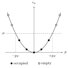
Schematic one-dimensional momentum cut through the three-dimensional free Fermi gas at $T=0$ and $\mu>0$. Filled and open circles illustrate occupied and empty modes on $\epsilon_p=p^2/(2m)$. The intersections at $p=\pm p_F$ satisfy $\epsilon_{p_F}=\mu$; no occupation at the boundary is prescribed. The drawing is not to scale and does not represent the three-dimensional density-of-states measure.

This is already a field-theoretic description of many-body physics. A huge number of particles is encoded by a simple occupation rule in momentum space. If each momentum also has a spin degeneracy $g_s$, the density formulas are multiplied by $g_s$; the spinless convention above keeps the algebra uncluttered.

Constant energy shifts

Sometimes one adds a constant one-particle energy $M$:

$$H_0\longrightarrow H_0+MN =\sum_{\mathbf p}\left(M+\frac{\mathbf p^2}{2m}\right)N_{\mathbf p}.$$

In a fixed-$N$ nonrelativistic problem, this only shifts all energies by the same constant $MN$. In a system where particle number can change, the shift is physical. In the grand-canonical ensemble, it can be absorbed into the chemical potential:

$$H_0+MN-\mu N=H_0-(\mu-M)N.$$

This is one reason nonrelativistic notation can hide a conceptual issue that returns in relativistic field theory. Once pair creation and antiparticles appear, the absolute one-particle energy and the mass gap become part of the structure of the theory.

Summary

The free nonrelativistic field is solved by Fourier transforming the local field operator into momentum modes. Each mode has a number operator $N_{\mathbf p}=a_{\mathbf p}^\dagger a_{\mathbf p}$, and the Hamiltonian is the sum of independent mode energies.

The same expression for $H_0$ applies to bosons and fermions, but the allowed occupation numbers are different. Bosons permit arbitrary occupation of a mode; fermions permit only $0$ or $1$. This microscopic algebraic distinction becomes macroscopic at finite density: free bosons accumulate in low-energy modes, while free fermions form a Fermi sea.

The next step is relativistic. The dispersion relation will become $\omega_{\mathbf p}=\sqrt{\mathbf p^2+m^2}$, and a local relativistic scalar field will contain both creation and annihilation operators. The free nonrelativistic field is the warm-up where the mode logic is completely visible.

Common pitfalls

The first trap is mixing box and continuum normalizations. In a box, $[a_{\mathbf p},a_{\mathbf q}^\dagger]_\eta=\delta_{\mathbf p\mathbf q}$. In the continuum, $[a(\mathbf p),a^\dagger(\mathbf q)]_\eta=(2\pi)^3\delta^{(3)}(\mathbf p-\mathbf q)$. The two are equivalent only if sums, integrals, delta functions, and operator normalizations are converted together.

The second trap is using anticommutators in the Heisenberg equation for fermions. For the fields and modes here, with no explicit Schrödinger-picture time dependence, the equation is $i\dot A=[A,H]$. Fermionic anticommutation relations enter when evaluating this ordinary commutator.

The third trap is confusing the field operator $\psi(\mathbf x,t)$ with a one-particle wavefunction. They satisfy the same free differential equation, but $\psi$ acts on Fock space and changes particle number.

The fourth trap is the sign of the chemical potential. With $K=H-\mu N$, filled fermion modes at zero temperature obey $\epsilon_{\mathbf p}<\mu$. Some references write $H+\mu N$; that is the same convention with the opposite sign for $\mu$.

Exercises

Exercise 1: recovering the periodic delta function

Show that the finite-box expansion

$$\psi(\mathbf x)=\frac1{\sqrt V}\sum_{\mathbf p}a_{\mathbf p}e^{i\mathbf p\cdot\mathbf x}$$

implies

$$[\psi(\mathbf x),\psi^\dagger(\mathbf y)]_\eta =\delta_V^{(3)}(\mathbf x-\mathbf y),$$

where

$$\delta_V^{(3)}(\mathbf x-\mathbf y) =\frac1V\sum_{\mathbf p}e^{i\mathbf p\cdot(\mathbf x-\mathbf y)}.$$

Solution

Using $[a_{\mathbf p},a_{\mathbf q}^\dagger]_\eta=\delta_{\mathbf p\mathbf q}$,

$$\begin{aligned} [\psi(\mathbf x),\psi^\dagger(\mathbf y)]_\eta &=\frac1V\sum_{\mathbf p,\mathbf q} e^{i\mathbf p\cdot\mathbf x}e^{-i\mathbf q\cdot\mathbf y} [a_{\mathbf p},a_{\mathbf q}^\dagger]_\eta \\ &=\frac1V\sum_{\mathbf p}e^{i\mathbf p\cdot(\mathbf x-\mathbf y)} =\delta_V^{(3)}(\mathbf x-\mathbf y). \end{aligned}$$

As $V\to\infty$, this becomes the ordinary Dirac delta function.

Exercise 2: deriving the momentum operator

Starting from

$$\mathbf P=\int d^3x\,\psi^\dagger(-i\nabla)\psi,$$

show that

$$\mathbf P=\sum_{\mathbf p}\mathbf p\,a_{\mathbf p}^\dagger a_{\mathbf p}.$$

Solution

Use

$$-i\nabla\psi(\mathbf x) =\frac1{\sqrt V}\sum_{\mathbf p}\mathbf p\,a_{\mathbf p}e^{i\mathbf p\cdot\mathbf x}.$$

Then

$$\begin{aligned} \mathbf P &=\frac1V\sum_{\mathbf p,\mathbf q}\mathbf p\,a_{\mathbf q}^\dagger a_{\mathbf p} \int d^3x\,e^{i(\mathbf p-\mathbf q)\cdot\mathbf x} \\ &=\sum_{\mathbf p}\mathbf p\,a_{\mathbf p}^\dagger a_{\mathbf p}. \end{aligned}$$

Each occupied mode contributes its momentum once per particle.

Exercise 3: spinless Fermi gas at zero temperature

For spinless fermions in three dimensions, prove

$$\frac EV=\frac35 n\epsilon_F, \qquad n=\frac{p_F^3}{6\pi^2}, \qquad \epsilon_F=\frac{p_F^2}{2m}.$$

Solution

The ground state fills the Fermi sphere:

$$\frac EV =\int_{|\mathbf p|<p_F}\frac{d^3p}{(2\pi)^3}\frac{p^2}{2m} =\frac{4\pi}{(2\pi)^3}\int_0^{p_F}dp\,p^2\frac{p^2}{2m}.$$

Therefore

$$\frac EV=\frac{p_F^5}{20\pi^2m}.$$

Since

$$n\epsilon_F=\frac{p_F^3}{6\pi^2}\frac{p_F^2}{2m} =\frac{p_F^5}{12\pi^2m},$$

we get

$$\frac EV=\frac35 n\epsilon_F.$$

Exercise 4: convergence of the free Bose mode

For a single bosonic mode, show that

$$Z=\sum_{n=0}^{\infty}e^{-\beta(\epsilon-\mu)n}$$

converges only for $\mu<\epsilon$.

Solution

The series is geometric with ratio

$$r=e^{-\beta(\epsilon-\mu)}.$$

It converges only if $r<1$, which gives

$$\epsilon-\mu>0.$$

Hence $\mu<\epsilon$. For a finite many-mode gas, this must hold for the lowest mode, so $\mu<\epsilon_{\mathrm{min}}$. In the thermodynamic Bose-condensed limit one takes $\mu\to\epsilon_{\mathrm{min}}$ from below and treats the lowest mode separately rather than summing it as a convergent geometric series.

References

• Coleman, Sidney. Lectures of Sidney Coleman on Quantum Field Theory. Edited by Bryan Gin-ge Chen, David Derbes, David Griffiths, Brian Hill, Richard Sohn and Yuan-Sen Ting. World Scientific, 2019. DOI.
• Srednicki, Mark. Quantum Field Theory. Prepublication author manuscript, 2006. Author’s page; Open PDF. The cited page numbers refer to this manuscript.