

Identical Particles and Fock Space
The oscillator algebra from the previous page already knows how to count quanta. What it does not yet explain is why this is the correct language for identical particles. In ordinary one-particle quantum mechanics, a state vector describes one object. In QFT, the Hilbert space must describe any number of quanta, and those quanta usually have no permanent individual labels.
For bosons, exchanging two particles does not change the state. The -particle wavefunction is symmetric,
and similarly in momentum space. The natural basis is therefore not a list of named particles, but a list of occupation numbers: how many particles occupy each one-particle state.
The bosonic Fock space is the direct sum of all symmetric -particle sectors,
Creation and annihilation operators move between adjacent sectors. They add or remove one particle in a chosen mode, and their commutation relations encode the symmetry factors that otherwise have to be inserted by hand.
The central reader’s trap is to carry over too much intuition from distinguishable particles. A bosonic Fock state is not a wavefunction for a collection of named objects. It is a vector whose components say which one-particle modes are occupied and how many times.
Identical bosons and symmetric states
Section titled “Identical bosons and symmetric states”Imagine two particles and two available one-particle levels, labeled and . If the particles were distinguishable, say particle and particle , then the ordered assignments would be
The two mixed assignments are different if the labels and are physical. For identical bosons, however, there is no physical experiment that tracks permanent labels and . The states are instead
Here means “two particles in level and none in level ,” while means “one particle in each level.” The order in which we name the particles has disappeared.
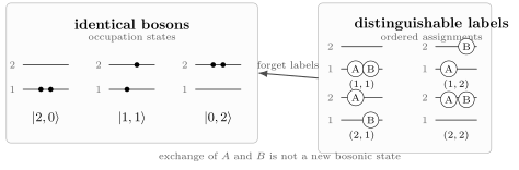
For two one-particle levels, two distinguishable particles have four ordered assignments. Two identical bosons have three occupation states: , , and . The two mixed ordered assignments differ only by exchanging labels, so they represent the same bosonic state.
This example is also a warning about probabilities. Statements such as “the probability of a configuration is ” or “the probability is ” are not universal facts; they depend on which ensemble is being declared equally likely. The universal statement is the state-counting statement: bosonic states are labeled by occupations, not by ordered particle labels.
Let be the one-particle Hilbert space. If particles carried physical labels, the -particle Hilbert space would be the full tensor product
A coordinate-space vector in this tensor product has wavefunction
For identical bosons, exchanging any pair of arguments must leave the wavefunction unchanged:
Thus the bosonic -particle sector is the symmetric subspace
where permutes the tensor factors. The symmetrization operator is
It is a projection:
For example, if and are orthonormal one-particle states with , the normalized two-boson state with one particle in each mode is
If both particles are in the same state , the state is simply
There is no extra factor of in this second formula, because is already normalized.
Counting occupation states
Section titled “Counting occupation states”Suppose there are one-particle levels and identical bosons. A bosonic state in the occupation basis is specified by nonnegative integers
The number of such occupation patterns is the stars-and-bars number
For ,
This is the number of independent symmetric coefficients in a two-particle wavefunction expanded as
The diagonal components describe double occupation of one level. The off-diagonal components with describe one particle in each of two different levels.
This replacement of ordered labels by occupation numbers is the first large simplification of many-particle quantum mechanics. Instead of carrying redundant information about which identical particle is which, the occupation basis keeps only the physical information. The same relabeling of bosonic basis states is developed in Coleman 2019, § 2.2, pp. 20–21.
Fock space
Section titled “Fock space”A fixed- Hilbert space is not enough for field theory. Interactions can create and annihilate quanta, and even when particle number happens to be conserved, the operator language is clearest when all sectors are present at once.
The bosonic Fock space over is
The vector is the vacuum, the unique state in the zero-particle sector. It is not the zero vector. It is a normalized physical state satisfying
A general Fock-space vector is a sequence
The total particle-number operator is
It acts diagonally:
A state with definite particle number lies entirely in one sector. A general Fock state may be a superposition of different particle numbers.
Creation and annihilation as maps between sectors
Section titled “Creation and annihilation as maps between sectors”Creation and annihilation operators can be described in two closely related languages. The unnormalized symmetric-list notation makes the combinatorics visible: annihilation literally counts how many matching entries can be removed. The normalized occupation notation is better for matrix elements, probabilities, and Hamiltonian eigenstates. Moving between these two languages is one of the basic skills of QFT.
More explicitly, define
Because the creation operators commute, this state depends only on the multiset of occupied modes, not on the order of the displayed labels. If mode occurs times, then in a discrete orthonormal basis its squared norm is
The subscript is therefore a reminder: these states are convenient algebraically, but are not generally normalized. Creation by a mode is written simply as
Annihilation removes one occurrence of from the list and sums over all places it could have been found:
The hat means that the entry is omitted. For a single mode this reduces to
Here the factor appears because there are identical quanta that could be removed.
The commutator follows immediately:
so
Since this holds for every ,
Normalized states are obtained by dividing out the factorials generated by repeated creation. For one mode,
Equivalently, if , then
The same operator actions become
For many modes,
where only finitely many are nonzero for a finite-particle state. Then
and
The mode number operator is
and
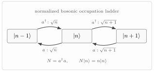
For normalized bosonic occupation states, raises the occupation number with coefficient , while lowers it with coefficient . In an unnormalized basis the same rules are and .
The square-root coefficients are not arbitrary conventions. They are the unique coefficients compatible with normalized states and the commutator .
Inner products and repeated momenta
Section titled “Inner products and repeated momenta”When all momenta are distinct, a symmetrized -particle state can be written as
This formula must be modified when some momenta are repeated, because the sum over permutations then repeats identical tensor products. The occupation-number formula avoids this trap automatically.
If the mode occurs times, the normalized occupation state is
In tensor-product notation, if is a list with occupation numbers , then the same normalized bosonic state can be written as
The extra factor compensates for repeated terms in the permutation sum. Check the two extremes: if all are distinct, every is or and the coefficient reduces to ; if all particles occupy the same mode, the permutation sum contains identical terms and the formula gives a single normalized tensor product. This is one of the places where occupation numbers are not merely convenient; they are safer than ordered particle labels.
Hamiltonian and wavefunctions in occupation language
Section titled “Hamiltonian and wavefunctions in occupation language”Let the one-particle Hamiltonian have eigenstates with energies :
The corresponding free many-boson Hamiltonian is
Acting on an occupation state,
In a relativistic momentum basis,
and therefore
A state with occupation numbers has energy
This is the additive many-particle spectrum, now written without naming the particles.
A vector in the -particle sector can also be represented by a coordinate-space wavefunction
or by a momentum-space wavefunction
For bosons both are symmetric:
and
For example, the normalized two-boson state with one particle in one-particle wavefunction and one in , with , has coordinate wavefunction
The same state in Fock notation is
where
The operator notation hides the symmetrization because the commutation relation already performs it. This is the main practical advantage of second quantization: the many-particle symmetry is built into the algebra, so calculations can focus on operators rather than repeatedly symmetrizing wavefunctions.
A two-level check
Section titled “A two-level check”Let the one-particle levels have energies and . The two-boson sector has three normalized occupation states:
and
The free Hamiltonian
has eigenvalues
and
Now act with :
The coefficient is not a mysterious interaction. It is the square root of the number of identical quanta available in mode .
Summary
Section titled “Summary”Fock space replaces particle labels by mode occupations. For bosons,
and the normalized occupation state is
Creation and annihilation act by
and
The free Hamiltonian is diagonal in this basis:
The physical lesson is sharper than the notation suggests. The statement “there are three bosons in mode ” is meaningful. The statement “this particular boson is particle number one” is not. Creation and annihilation operators are the linear maps that respect this fact.
Common pitfalls
Section titled “Common pitfalls”Treating exchange as a physical motion
Section titled “Treating exchange as a physical motion”Exchange symmetry is not the statement that two particles physically travel around each other. It is a statement about how the state is represented when two identical arguments or labels are interchanged. For bosons, the state is invariant under this relabeling.
Confusing symmetric states with product states
Section titled “Confusing symmetric states with product states”The state
is not the same vector as in the full tensor product. It lies in the symmetric subspace. The occupation notation automatically means the symmetric state.
Forgetting normalization when particles occupy the same mode
Section titled “Forgetting normalization when particles occupy the same mode”The normalized state with two bosons in the same mode is
Dropping the gives an unnormalized state. That may be harmless in a short algebraic derivation if one is consistent, but it gives wrong matrix elements if used as a normalized state.
Assuming Bose counting fixes probabilities by itself
Section titled “Assuming Bose counting fixes probabilities by itself”Bose symmetry tells us which states are distinct. It does not by itself determine a probability distribution over those states. Probabilities require dynamics, a density matrix, or an ensemble assumption.
Mixing fixed-particle and Fock-space notation
Section titled “Mixing fixed-particle and Fock-space notation”A wavefunction lives in a fixed -particle sector. A Fock vector contains all sectors at once. Operators like and move between sectors, so they are not operators on a single fixed- Hilbert space alone.
The Library treatment of Multiparticle States, Statistics, and Fock Organization develops the symmetric and antisymmetric tensor spaces underlying this lesson’s occupation-number construction, including normalization and fermionic ordering.
Exercises
Section titled “Exercises”Exercise 1: counting bosonic states
Section titled “Exercise 1: counting bosonic states”Show that the number of ways to put identical bosons into one-particle levels is
Check explicitly that for and the answer is .
Solution
A bosonic occupation state is specified by nonnegative integers
This is the standard stars-and-bars problem. Represent the particles as stars and use bars to separate the levels. For example, with ,
represents . There are stars and bars, so there are slots in total. Choosing the slots occupied by stars gives
For and ,
The six states are
Exercise 2: deriving the ladder coefficients
Section titled “Exercise 2: deriving the ladder coefficients”Starting from
show that
Solution
For creation,
Since
we have
For annihilation, use
Acting on the vacuum removes the first term because , so
Using
we get
Exercise 3: annihilation from an unnormalized symmetric list
Section titled “Exercise 3: annihilation from an unnormalized symmetric list”Let
be an unnormalized symmetric momentum state. Use
to compute and for .
Solution
First remove a particle of momentum :
Since , this becomes
Now remove a particle of momentum :
Again using ,
The factor appears because there are two identical entries with momentum that can be removed.
Exercise 4: two-boson wavefunction from operators
Section titled “Exercise 4: two-boson wavefunction from operators”Let and be orthonormal one-particle wavefunctions. Define
where and . Show that the state
corresponds to the normalized symmetric coordinate wavefunction
Solution
In an unsymmetrized tensor product, the product state with one particle in and one in would be
For identical bosons we must project to the symmetric subspace:
Because and are orthonormal, the norm of the numerator is
Thus the normalized state is
Taking the coordinate-space matrix element gives
The operator state gives exactly this vector because the creation operators commute:
So the ordering of creation is not a physical label; it only constructs the symmetric state.
References
Section titled “References”- Coleman, Sidney. Lectures of Sidney Coleman on Quantum Field Theory. Edited by Bryan Gin-ge Chen, David Derbes, David Griffiths, Brian Hill, Richard Sohn, and Yuan-Sen Ting. World Scientific, 2019. DOI: 10.1142/9371. § 2.2, pp. 20–21, constructs the occupation-number labeling of bosonic states.
Further reading
Section titled “Further reading”- Peskin, Michael E., and Daniel V. Schroeder. An Introduction to Quantum Field Theory. Addison-Wesley, 1995. Publisher. Chapter 2 develops creation and annihilation operators for the free scalar field.
- Schwartz, Matthew D. Quantum Field Theory and the Standard Model. Cambridge University Press, 2014. DOI: 10.1017/9781139540940. Chapter 2 introduces the oscillator description of quantum fields.
- Srednicki, Mark. Quantum Field Theory. Cambridge University Press, 2007. DOI: 10.1017/CBO9780511813917. Chapters 2–4 provide the relativistic scalar-field setting.
- Weinberg, Steven. The Quantum Theory of Fields, Volume I: Foundations. Cambridge University Press, 1995. DOI: 10.1017/CBO9781139644167. Chapters 2, 4, and 5 develop multiparticle states, creation operators, and quantum fields.