Perturbation Theory from Functional Derivatives

The source functional introduced on the previous page gives a compact description of free Green functions. For a Gaussian theory, differentiating

$$Z_0[J]=\exp\left[-\frac12\int d^dx\,d^dy\,J(x)G_0(x,y)J(y)\right]$$

reproduces Wick theorem: every pair of source derivatives produces one propagator. The next step is the real reason this notation is so useful. An interaction is a polynomial in the field, and a field insertion is generated by $(1/i)\delta/\delta J$. Therefore the interacting path integral can be generated by applying a differential operator to the free Gaussian.

This page develops that statement carefully. It connects three viewpoints that are often taught separately: the Dyson expansion in the interaction picture, the source-functional expansion, and the diagrammatic rules for the first perturbative corrections. The central point is that Feynman diagrams are not a new formalism; they are the bookkeeping device that records functional derivatives acting on a Gaussian.

The reader should leave this page able to do two practical things: translate an interaction term into a differential operator acting on $Z_0[J]$, and read the coefficient of a first-order diagram without guessing the symmetry factor from memory.

We write $G_0(x,y)$ for the free Feynman propagator denoted $G_F(x-y)$ on the previous page. In a translationally invariant vacuum,

$$G_0(x,y)=G_F(x-y),$$

so the change of notation only makes the two endpoints explicit. This page works in $d$ spacetime dimensions; the preceding four-dimensional formulas are recovered by setting $d=4$.

The Green-function hierarchy

Lorentzian interaction and vertex normalization

We use a real Lorentzian scalar field with

$$S[\phi]=S_0[\phi]+S_{\mathrm{int}}[\phi], \qquad S_{\mathrm{int}}[\phi]=-\int d^dx\,V(\phi(x)).$$

For the main example,

$$V(\phi)=\frac{\lambda}{4!}\phi^4, \qquad V'(\phi)=\frac{\lambda}{3!}\phi^3.$$

The source coupling is $+\int J\phi$, so each insertion of $\phi(x)$ is generated by $(1/i)\delta/\delta J(x)$. With these conventions a single $\phi^4$ vertex contributes the Lorentzian factor $-i\lambda$ before symmetry factors.

Before writing any diagrams, it is useful to see what perturbation theory is trying to solve. The classical equation of motion for

$$S=\int d^dx\left[\frac12\partial_\mu\phi\partial^\mu\phi-\frac12m^2\phi^2-V(\phi)\right]$$

is

$$(\Box+m^2)\phi(x)+V'(\phi(x))=0.$$

The quantum identities below are exact statements of a regulated theory. When $V'(\phi)$ contains coincident products such as $\phi^3(x)$, that composite operator must be defined with the same regulator and, in the continuum limit, generally requires renormalization.

Inside a time-ordered quantum correlator, this equation receives contact terms when the differential operator hits the time ordering. For the two-point function,

$$\boxed{ (\Box_{x_1}+m^2)\langle\mathcal T\phi(x_1)\phi(x_2)\rangle +\langle\mathcal T V'(\phi(x_1))\phi(x_2)\rangle =-i\delta^{(d)}(x_1-x_2). }$$

For $V(\phi)=\lambda\phi^4/4!$, this becomes

$$(\Box_{x_1}+m^2)G_2(x_1,x_2) +\frac{\lambda}{3!}\langle\mathcal T\phi^3(x_1)\phi(x_2)\rangle =-i\delta^{(d)}(x_1-x_2).$$

The equation is exact, but it is not closed. The two-point function depends on a four-point function. Acting on that four-point function produces a six-point function, and so on. The previous page derived the underlying integration-by-parts identity; this short hierarchy discussion shows what perturbation theory is solving, and the next page revisits the hierarchy systematically. More generally,

$$\boxed{ \begin{aligned} &(\Box_{x_1}+m^2)G_n(x_1,\ldots,x_n) +\langle\mathcal T V'(\phi(x_1))\phi(x_2)\cdots\phi(x_n)\rangle \\ &\qquad =-i\sum_{j=2}^n\delta^{(d)}(x_1-x_j) G_{n-2}(x_2,\ldots,\widehat{x_j},\ldots,x_n). \end{aligned} }$$

The hat means that the argument is omitted. This infinite chain is the Schwinger–Dyson hierarchy in its equation-of-motion form. Perturbation theory solves it by expanding the higher correlators in powers of the interaction and reducing each term to free Wick contractions.

The functional derivative method gives the most economical way to do this reduction.

Interactions as differential operators

Start from the normalized generating functional

$$Z[J]=\frac{\displaystyle\int\mathcal D\phi\, \exp\left(iS_0[\phi]+iS_{\mathrm{int}}[\phi]+i\int d^dx\,J(x)\phi(x)\right)} {\displaystyle\int\mathcal D\phi\, \exp\left(iS_0[\phi]+iS_{\mathrm{int}}[\phi]\right)}.$$

The denominator enforces $Z[0]=1$. Since

$$\frac{1}{i}\frac{\delta}{\delta J(x)} \exp\left(i\int d^dy\,J(y)\phi(y)\right) =\phi(x) \exp\left(i\int d^dy\,J(y)\phi(y)\right),$$

any polynomial in $\phi$ can be replaced, under the path integral, by the same polynomial in $(1/i)\delta/\delta J$. Thus

$$\int\mathcal D\phi\,e^{iS_0[\phi]+i\int J\phi} \,e^{iS_{\mathrm{int}}[\phi]} = \exp\left(iS_{\mathrm{int}}\left[\frac1i\frac{\delta}{\delta J}\right]\right) \int\mathcal D\phi\,e^{iS_0[\phi]+i\int J\phi}.$$

After dividing by the same expression at $J=0$, the exact formal result is

$$\boxed{ Z[J] = \frac{\displaystyle \exp\left(iS_{\mathrm{int}}\left[\frac1i\frac{\delta}{\delta J}\right]\right)Z_0[J]} {\displaystyle \left.\exp\left(iS_{\mathrm{int}}\left[\frac1i\frac{\delta}{\delta J}\right]\right)Z_0[J]\right|_{J=0}}. }$$

For $\phi^4$ theory this becomes

$$\boxed{ Z[J] = \frac{\displaystyle \exp\left[-\frac{i\lambda}{4!}\int d^dx\, \left(\frac1i\frac{\delta}{\delta J(x)}\right)^4\right]Z_0[J]} {\displaystyle \left.\exp\left[-\frac{i\lambda}{4!}\int d^dx\, \left(\frac1i\frac{\delta}{\delta J(x)}\right)^4\right]Z_0[J]\right|_{J=0}}. }$$

A useful sign check is that $(1/i)^4=1$, so the Lorentzian vertex sign comes entirely from the factor $iS_{\mathrm{int}}=-i\lambda\int\phi^4/4!$. The $4!$ in the denominator is not a vertex factor by itself; it is canceled partly or completely by the number of Wick contractions that produce the diagram under study.

The perturbation series is obtained by expanding the exponential in powers of $\lambda$. Each power introduces one or more integration points, which become vertices. The functional derivatives at each vertex act on the Gaussian $Z_0[J]$, and because $Z_0[J]$ is quadratic in $J$, every surviving term is a sum of pairwise contractions.

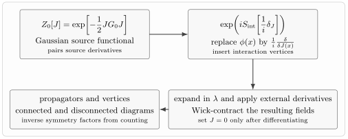
The free Gaussian $Z_0[J]$ generates propagators. The interaction $S_{\mathrm{int}}[\phi]$ becomes the differential operator $S_{\mathrm{int}}[(1/i)\delta_J]$. Expanding this operator produces vertices, and differentiating with respect to external sources attaches external fields.

The $n$-point functions are still generated by

$$G_n(x_1,\ldots,x_n) =\left.\frac{1}{i^n}\frac{\delta^nZ[J]} {\delta J(x_1)\cdots\delta J(x_n)}\right|_{J=0}.$$

The formula is compact, but it contains all the usual perturbative ingredients: propagators, vertices, integration over internal points, external insertions, and symmetry factors.

For actual calculations it is helpful to keep the following dictionary in mind. Source derivatives placed outside the interaction operator create the external fields of the requested Green function. Source derivatives inside $S_{\mathrm{int}}[(1/i)\delta_J]$ create the fields sitting at an interaction vertex. After all derivatives act on the Gaussian, every pair of differentiated sources is replaced by a free propagator. The final instruction $J=0$ discards any term with an unpaired source.

Relation to the interaction picture

The same expansion appears in operator language. Let

$$H=H_0+H_{\mathrm{int}},$$

and define interaction-picture fields by

$$\phi_I(t,\mathbf x)=e^{iH_0t}\phi(0,\mathbf x)e^{-iH_0t}.$$

The interaction-picture evolution operator is

$$U(t,t_0) =\mathcal T\exp\left[-i\int_{t_0}^t d\tau\,H_I(\tau)\right].$$

To compute vacuum correlation functions in the interacting theory, one must also prepare the interacting vacuum. This is done by turning on the interaction adiabatically, for example by replacing $H_I(t)$ with $e^{-\epsilon |t|}H_I(t)$ and taking $\epsilon\to0^+$ at the end. The resulting Gell-Mann–Low formula is

$$\boxed{ \langle\Omega|\mathcal T\phi_H(x_1)\cdots\phi_H(x_n)|\Omega\rangle = \lim_{\epsilon\to0^+} \frac{\langle0|\mathcal T\phi_I(x_1)\cdots\phi_I(x_n) \exp\left[-i\int d^dz\,e^{-\epsilon|z^0|}\mathcal H_I(z)\right]|0\rangle} {\langle0|\mathcal T \exp\left[-i\int d^dz\,e^{-\epsilon|z^0|}\mathcal H_I(z)\right]|0\rangle}. }$$

Here $|0\rangle$ is the free vacuum and $|\Omega\rangle$ is the interacting vacuum. The displayed limit makes explicit the adiabatic switch that is often suppressed in the Gell-Mann–Low formula. The denominator is the operator version of the normalization of $Z[J]$; it cancels vacuum bubbles.

For a scalar interaction $V(\phi)=\lambda\phi^4/4!$, the interaction Hamiltonian density is

$$\mathcal H_I(x)=\frac{\lambda}{4!}\phi_I^4(x),$$

so the exponential is

$$\exp\left[-\frac{i\lambda}{4!}\int d^dx\,\phi_I^4(x)\right].$$

This is the same object that appeared in the source-functional formula, with each $\phi_I(x)$ replaced by $(1/i)\delta/\delta J(x)$. The path-integral and operator derivations are therefore not competing stories. They are two ways of organizing the same Dyson expansion.

The two-point function at first order

Let

$$G_2(x_1,x_2)=\langle\Omega|\mathcal T\phi(x_1)\phi(x_2)|\Omega\rangle.$$

Expanding the normalized expectation value to first order in $\lambda$ gives

$$\begin{aligned} G_2(x_1,x_2) &=G_0(x_1,x_2) -\frac{i\lambda}{4!}\int d^dz\, \langle\mathcal T\phi(x_1)\phi(x_2)\phi^4(z)\rangle_0 \\ &\qquad +G_0(x_1,x_2)\frac{i\lambda}{4!}\int d^dz\, \langle\mathcal T\phi^4(z)\rangle_0 +O(\lambda^2). \end{aligned}$$

The last term comes from expanding the denominator. It subtracts the vacuum bubble disconnected from the external fields.

Now apply Wick theorem. The free six-point function contains two types of contractions. First, the two external fields may contract with each other, while the four fields at $z$ form a vacuum bubble:

$$\langle\mathcal T\phi(x_1)\phi(x_2)\phi^4(z)\rangle_0 \supset 3G_0(x_1,x_2)G_0(z,z)^2.$$

This is precisely canceled by the denominator. Second, one field at $z$ contracts with $x_1$, another field at $z$ contracts with $x_2$, and the remaining two fields at $z$ contract with each other. There are

$$4\cdot3=12$$

such contractions. Therefore the connected first-order correction is

$$\boxed{ G_2^{(1)}(x_1,x_2) =-\frac{i\lambda}{2}\int d^dz\, G_0(x_1,z)G_0(z,z)G_0(z,x_2). }$$

The diagram has symmetry factor $S=2$, so its diagrammatic weight is the inverse symmetry factor

$$\frac1S=\frac12=\frac{12}{4!}.$$

Notice what is being computed: $G_2^{(1)}$ is an unamputated Green-function correction. The two outer propagators describe propagation from $x_1$ to the vertex and from the vertex to $x_2$. The amputated middle factor is what will later be isolated as a self-energy insertion.

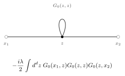
The first correction to the two-point function in $\phi^4$ theory is a tadpole insertion. The two external propagators attach to the interaction point $z$, while two fields at the same vertex contract with each other to form $G_0(z,z)$.

In continuum field theory the factor $G_0(z,z)$ is usually ultraviolet divergent. This is not a failure of the expansion. It is the first visible sign that local parameters in the Lagrangian, especially the mass, must be renormalized.

The four-point function at first order

The four-point function shows even more clearly how diagrams emerge from functional derivatives. At zeroth order,

$$G_4^{(0)}(x_1,x_2,x_3,x_4) =G_0(x_1,x_2)G_0(x_3,x_4) +G_0(x_1,x_3)G_0(x_2,x_4) +G_0(x_1,x_4)G_0(x_2,x_3).$$

This is just Wick theorem. At first order, the connected part comes from attaching all four external fields to one interaction vertex:

$$G_{4,\mathrm{conn}}^{(1)}(x_1,x_2,x_3,x_4) =-\frac{i\lambda}{4!}\int d^dz\, \left.\langle\mathcal T\phi(x_1)\phi(x_2)\phi(x_3)\phi(x_4)\phi^4(z)\rangle_0 \right|_{\text{all external fields attached to }z}.$$

The restriction selects Wick pairings that become connected after the four fields at $z$ are identified as one interaction vertex; it does not mean that the free Gaussian theory has a nonzero connected eight-point cumulant. There are $4!$ ways to connect the four fields at $z$ to the four external points, so the $4!$ in the interaction cancels:

$$\boxed{ G_{4,\mathrm{conn}}^{(1)}(x_1,x_2,x_3,x_4) =-i\lambda\int d^dz\, G_0(x_1,z)G_0(x_2,z)G_0(x_3,z)G_0(x_4,z). }$$

The full four-point function at this order also contains disconnected terms: one of the three free Wick pairings may receive the tadpole correction derived above, while the other pair remains a free propagator. Schematically,

$$G_4^{(1)}=G_{4,\mathrm{conn}}^{(1)} +\sum_{\{(ij),(k\ell)\}\in\mathcal P_2(4)} \left(G_2^{(1)}(x_i,x_j)G_0(x_k,x_\ell) +G_0(x_i,x_j)G_2^{(1)}(x_k,x_\ell)\right).$$

Here $\mathcal P_2(4)$ is the set of the three unordered partitions of four labels into two pairs. For each partition there are two choices for which pair carries the tadpole correction, giving six disconnected terms in total.

The connected four-point diagram is the first place where the interaction creates a genuinely new four-field correlation rather than merely correcting a propagator. It is still an unamputated Green function, not yet an $S$-matrix element. Scattering amplitudes are obtained only after putting external legs on shell and amputating their propagators.

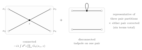
At order $\lambda$, the four-point function contains a connected vertex diagram and disconnected pieces in which one free propagator is corrected by a tadpole while the other propagator remains free. The three pair partitions and the choice of which pair is corrected give six disconnected terms. Connected Green functions keep only the first topology.

Vacuum bubbles and why the denominator matters

The normalized functional

$$Z[J] =\frac{\int\mathcal D\phi\,e^{iS+i\int J\phi}} {\int\mathcal D\phi\,e^{iS}}$$

is not just aesthetically pleasing. Without the denominator, every correlator would be multiplied by diagrams that live entirely in the vacuum and are disconnected from all external insertions.

To see the cancellation explicitly, write the numerator for an operator $\mathcal O$ as

$$N_{\mathcal O}=\langle\mathcal O\rangle_0 +N_{\mathcal O}^{(1)}+O(\lambda^2),$$

and the vacuum denominator as

$$D=1+D^{(1)}+O(\lambda^2).$$

Then

$$\frac{N_{\mathcal O}}{D} =\langle\mathcal O\rangle_0 +N_{\mathcal O}^{(1)}- \langle\mathcal O\rangle_0D^{(1)}+O(\lambda^2).$$

The term $\langle\mathcal O\rangle_0D^{(1)}$ subtracts exactly the first-order vacuum bubble attached to the free correlator by multiplication. The same cancellation persists to all orders: diagrams disconnected from every external source exponentiate and cancel between numerator and denominator.

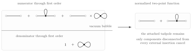
The denominator in the normalized generating functional cancels vacuum bubbles. After this cancellation, perturbative correlators contain diagrams connected to the external insertions, plus products of such connected components when the full rather than connected Green function is requested.

This is why the logarithm $W[J]=-i\log Z[J]$ generates connected diagrams. Normalizing $Z[J]$ removes vacuum bubbles; taking $\log Z[J]$ removes products of disconnected source-connected components.

From formulas to diagrammatic rules

The functional derivative expansion immediately gives the coordinate-space Feynman rules for the scalar theory with $V(\phi)=\lambda\phi^4/4!$:

1. Draw external points $x_1,\ldots,x_n$ for the fields in the Green function.
2. For each power of the interaction, introduce an internal vertex point $z$ and integrate over it with $\int d^dz$.
3. Attach four line ends to each $\phi^4$ vertex.
4. Each line connecting points $a$ and $b$ contributes a free propagator $G_0(a,b)$.
5. Each vertex contributes $-i\lambda$.
6. Divide by the symmetry factor left over from automorphisms of the diagram.
7. Drop vacuum bubbles in normalized correlators; keep disconnected source-connected pieces only if computing the full $G_n$ rather than the connected function.

The phrase “symmetry factor” can sound like a mysterious diagrammatic correction. It is not. For fixed, labeled external insertions, suppose a topology with $n$ identical $\phi^4$ vertices is produced by $N_{\mathrm{contr}}$ Wick contractions. Then

$$\frac1S=\frac{N_{\mathrm{contr}}}{n!(4!)^n}$$

is its inverse symmetry factor. A reliable workflow is: first label every field, count contractions, multiply by the expansion factors, and only then translate the result into an unlabeled diagram.

For example, the two-point tadpole had $12$ Wick contractions and a prefactor $1/4!$, leaving the weight $1/S=12/24=1/2$, so $S=2$. The connected four-point vertex had $4!$ Wick contractions and a prefactor $1/4!$, leaving $1/S=1$.

Summary

Perturbation theory from sources is built on one substitution:

$$\phi(x)\longrightarrow \frac1i\frac{\delta}{\delta J(x)}.$$

Since the free source functional is Gaussian, functional derivatives acting on $Z_0[J]$ reproduce Wick contractions. Since interactions are polynomials in $\phi$, they become polynomial differential operators acting on $Z_0[J]$. This turns the interacting generating functional into

$$Z[J] = \frac{e^{iS_{\mathrm{int}}[(1/i)\delta_J]}Z_0[J]} {\left.e^{iS_{\mathrm{int}}[(1/i)\delta_J]}Z_0[J]\right|_{J=0}}.$$

Expanding this formula gives the Dyson series, but in a form that automatically generates diagrams. The denominator cancels vacuum bubbles. The logarithm generates connected diagrams. The first nontrivial examples in $\phi^4$ theory are the tadpole correction to the two-point function and the connected four-point vertex.

The page also reveals why interacting Green functions form a hierarchy. The equation of motion for $G_2$ contains $\langle\mathcal T\phi^3\phi\rangle$; higher equations contain still higher correlators. Perturbation theory closes this hierarchy order by order by reducing every interacting insertion to free propagators.

Common pitfalls

Do not apply $S_{\mathrm{int}}[(1/i)\delta_J]$ to $\log Z_0[J]$. The interaction differential operator acts on $Z_0[J]$ itself. Connected diagrams emerge only after normalization and then taking the logarithm.

Do not forget the denominator in the Gell-Mann–Low formula or in $Z[J]$. It is responsible for canceling vacuum bubbles. Omitting it gives correct connected diagrams only by accident in very simple examples.

Do not assign the factor $-i\lambda/2$ to every tadpole by memory. It is specific to the two-point tadpole in $\phi^4$ theory with the normalization $\lambda\phi^4/4!$. Different interactions and different diagram topologies have different symmetry factors.

Do not confuse the full four-point function with the connected four-point function. The full $G_4$ contains disconnected pairings and corrected pairings; the connected part is the piece that cannot be split into a product of lower correlators.

Do not ignore coincident propagators such as $G_0(z,z)$. They are often ultraviolet divergent in field theory and are not harmless constants. Their local structure is what later becomes mass renormalization.

Exercises

Exercise 1

Show directly that for

$$S_{\mathrm{int}}[\phi]=-\frac{\lambda}{4!}\int d^dx\,\phi^4(x),$$

the interacting generating functional can be written as

$$Z[J] =\frac{\displaystyle \exp\left[-\frac{i\lambda}{4!}\int d^dx\, \left(\frac1i\frac{\delta}{\delta J(x)}\right)^4\right]Z_0[J]} {\displaystyle \left.\exp\left[-\frac{i\lambda}{4!}\int d^dx\, \left(\frac1i\frac{\delta}{\delta J(x)}\right)^4\right]Z_0[J]\right|_{J=0}}.$$

Solution

Use

$$\frac1i\frac{\delta}{\delta J(x)}e^{i\int J\phi} =\phi(x)e^{i\int J\phi}.$$

Applying this four times gives

$$\left(\frac1i\frac{\delta}{\delta J(x)}\right)^4e^{i\int J\phi} =\phi^4(x)e^{i\int J\phi}.$$

Therefore the interaction factor inside the path integral may be replaced by

$$\exp\left[-\frac{i\lambda}{4!}\int d^dx\, \phi^4(x)\right] \longrightarrow \exp\left[-\frac{i\lambda}{4!}\int d^dx\, \left(\frac1i\frac{\delta}{\delta J(x)}\right)^4\right].$$

The remaining path integral is the free source functional $Z_0[J]$, up to the same normalization at $J=0$. Dividing by the $J=0$ expression gives the stated formula.

Exercise 2

Compute the combinatorial factor of the first-order two-point tadpole in $\phi^4$ theory. In other words, show that

$$-\frac{i\lambda}{4!}\int d^dz\, \left.\langle\mathcal T\phi(x_1)\phi(x_2)\phi^4(z)\rangle_0 \right|_{\text{both external fields attached to }z} =-\frac{i\lambda}{2}\int d^dz\,G_0(x_1,z)G_0(z,z)G_0(z,x_2).$$

Solution

The four fields at the vertex are identical. To make a connected correction to the two-point function, choose one of the four fields at $z$ to contract with $\phi(x_1)$ and one of the remaining three fields at $z$ to contract with $\phi(x_2)$. The remaining two fields at $z$ contract with each other.

The number of such contractions is

$$4\cdot3=12.$$

Thus

$$\left.\langle\mathcal T\phi(x_1)\phi(x_2)\phi^4(z)\rangle_0 \right|_{\text{both external fields attached to }z} =12G_0(x_1,z)G_0(x_2,z)G_0(z,z).$$

Multiplying by the prefactor gives

$$-\frac{i\lambda}{4!}\cdot12 =-\frac{i\lambda}{2}.$$

Since $G_0(x_2,z)=G_0(z,x_2)$ for a real scalar field, the result follows.

Exercise 3

Show that the connected order-$\lambda$ four-point function in $\phi^4$ theory is

$$G_{4,\mathrm{conn}}^{(1)}(x_1,x_2,x_3,x_4) =-i\lambda\int d^dz\,\prod_{a=1}^4G_0(x_a,z).$$

Solution

At first order,

$$G_{4,\mathrm{conn}}^{(1)} =-\frac{i\lambda}{4!}\int d^dz\, \left.\langle\mathcal T\phi(x_1)\phi(x_2)\phi(x_3)\phi(x_4)\phi^4(z)\rangle_0 \right|_{\text{all external fields attached to }z}.$$

A connected contraction must attach each external field to one of the four fields at $z$. There are $4!$ bijections between the four external fields and the four fields at the vertex. Each produces the same product

$$G_0(x_1,z)G_0(x_2,z)G_0(x_3,z)G_0(x_4,z).$$

The factor $4!$ from the contractions cancels the $4!$ in the interaction, leaving

$$G_{4,\mathrm{conn}}^{(1)} =-i\lambda\int d^dz\,\prod_{a=1}^4G_0(x_a,z).$$

Exercise 4

At order $\lambda$, show explicitly how the denominator cancels the vacuum-bubble contribution to the two-point function.

Solution

The numerator through first order is

$$N=G_0(x_1,x_2) -\frac{i\lambda}{4!}\int d^dz\, \langle\mathcal T\phi(x_1)\phi(x_2)\phi^4(z)\rangle_0.$$

The denominator is

$$D=1-\frac{i\lambda}{4!}\int d^dz\, \langle\mathcal T\phi^4(z)\rangle_0.$$

Since $1/D=1+\frac{i\lambda}{4!}\int d^dz\,\langle\phi^4(z)\rangle_0+O(\lambda^2)$,

$$\frac{N}{D} =G_0(x_1,x_2) -\frac{i\lambda}{4!}\int d^dz\, \langle\phi(x_1)\phi(x_2)\phi^4(z)\rangle_0 +\frac{i\lambda}{4!}G_0(x_1,x_2)\int d^dz\,\langle\phi^4(z)\rangle_0.$$

The part of the six-point Wick contraction in which $x_1$ contracts with $x_2$ and the four fields at $z$ contract among themselves is

$$G_0(x_1,x_2)\langle\phi^4(z)\rangle_0.$$

It is canceled by the last term. Therefore only contractions connected to the external points survive.

Exercise 5

For the interaction $V(\phi)=\lambda\phi^4/4!$, derive the first equation in the Green-function hierarchy,

$$(\Box_{x_1}+m^2)G_2(x_1,x_2) +\frac{\lambda}{3!}\langle\mathcal T\phi^3(x_1)\phi(x_2)\rangle =-i\delta^{(d)}(x_1-x_2).$$

Solution

The classical equation of motion is

$$(\Box+m^2)\phi(x)+\frac{\lambda}{3!}\phi^3(x)=0.$$

In a time-ordered product, applying $(\Box_{x_1}+m^2)$ to $\langle\mathcal T\phi(x_1)\phi(x_2)\rangle$ acts on the field and also on the step functions hidden in $\mathcal T$. The latter produces the same contact term as in the free theory, because it is fixed by the equal-time canonical commutator:

$$(\Box_{x_1}+m^2)\langle\mathcal T\phi(x_1)\phi(x_2)\rangle = -\frac{\lambda}{3!}\langle\mathcal T\phi^3(x_1)\phi(x_2)\rangle -i\delta^{(d)}(x_1-x_2).$$

Moving the interaction term to the left gives the desired identity.

References and further reading

• Mark Srednicki, Quantum Field Theory, Sections 8–10, for path integrals in free and interacting scalar field theory and the derivation of Feynman rules.
• Sidney Coleman, Lectures of Sidney Coleman on Quantum Field Theory, Chapters 7–8 and 28, for the interaction picture, Dyson formula, Wick diagrams, and functional integrals.
• Steven Weinberg, The Quantum Theory of Fields, Volume I, Chapter 9, for path-integral methods and the relation between source insertions and perturbation theory.
• A. Zee, Quantum Field Theory in a Nutshell, Appendix A and the early chapters on Feynman diagrams, for Gaussian identities and diagrammatic intuition.