QED as an Effective Field Theory

The previous pages developed renormalization in a deliberately general language: local operators, running couplings, anomalous dimensions, and Callan–Symanzik equations. We now specialize that language to a theory everyone knows but that is easy to underestimate: quantum electrodynamics.

The minimal QED Lagrangian is not the whole story. It is the beginning of a Wilsonian expansion. Once we decide to describe physics below some short-distance scale $\Lambda$, locality and gauge invariance allow an infinite tower of operators. The familiar renormalizable terms are the first terms in this tower; Pauli magnetic-moment terms, four-fermion interactions, higher-derivative photon terms, and nonlinear photon interactions are the later terms.

This viewpoint changes the question from “Which interactions are renormalizable?” to the more physical question “Which local interactions are important at the scale being probed?” QED is then not merely a fundamental-looking theory with a small coupling. It is a low-energy organizing principle: charge conservation, gauge redundancy, locality, and dimensional analysis tell us which mistakes are small.

Required background. Callan–Symanzik equations and marginal operators supplies the running-coupling and relevance conventions used to order the QED action. Helpful background. Wilsonian RG and operator mixing explains why integrating out short-distance modes generates a complete local operator basis rather than only the terms present in a microscopic Lagrangian.

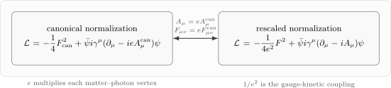
The electric charge may be placed either in the matter vertex or in the coefficient of the gauge kinetic term. The second convention makes the Wilsonian interpretation of $1/e^2$ as a local coupling especially transparent.

The effective Lagrangian viewpoint

Gauge-field normalization used below. In canonical normalization, QED is

$$\mathcal L_{\rm can} =-{1\over4}F^{\rm can}_{\mu\nu}F_{\rm can}^{\mu\nu} +\bar\psi\left(i\gamma^\mu(\partial_\mu-ieA^{\rm can}_\mu)-m\right)\psi$$

for a unit positively charged fermion. Equivalently, one may absorb the electric charge into the gauge field,

$$A_\mu=eA^{\rm can}_\mu, \qquad F_{\mu\nu}=eF^{\rm can}_{\mu\nu},$$

so that

$$\mathcal L =-{1\over4e^2}F_{\mu\nu}F^{\mu\nu} +\bar\psi\left(i\gamma^\mu D_\mu-m\right)\psi, \qquad D_\mu=\partial_\mu-iA_\mu.$$

This second convention is especially convenient for Wilsonian discussions because charge renormalization appears as renormalization of the coefficient of $F^2$. A unit positively charged field transforms as $\psi\mapsto e^{+i\alpha}\psi$ and uses $D_\mu=\partial_\mu-iA_\mu$. A field of charge $q$ uses $D_\mu=\partial_\mu-iqA_\mu$. Euclidean formulas differ by the usual Wick-rotation signs, but the operator hierarchy is unchanged.

How to read the QED EFT tower

The operator tower should be read as an error estimate. If an experiment probes momenta $E\ll\Lambda$, a dimension-$\Delta$ operator contributes schematically as

$$\Delta\mathcal A_\Delta\sim c_\Delta\left({E\over\Lambda}\right)^{\Delta-4}$$

relative to a dimension-four interaction with the same external fields, up to loop factors and symmetry factors. Thus a dimension-five Pauli term is the leading correction to magnetic-moment physics, while dimension-six four-fermion operators are the leading local remnants of heavy neutral or charged mediators. Gauge invariance tells us which operators are allowed; power counting tells us which allowed mistakes are numerically important.

Fix a scale $\Lambda$ above the momenta we intend to probe. The Wilsonian effective action is the most general local action consistent with the symmetries, organized as an expansion in powers of $E/\Lambda$, where $E$ is a typical external energy or momentum. For one charged Dirac fermion, we write schematically

$$\mathcal L_{\rm eff} =\mathcal L_{\rm QED}^{(4)}+ \sum_i {c_i\over \Lambda^{\Delta_i-4}}\mathcal O_i, \qquad \Delta_i>4.$$

Here $\Delta_i$ is the engineering dimension of $\mathcal O_i$ in four spacetime dimensions, and the coefficients $c_i$ are dimensionless Wilson coefficients. They may contain logarithms, group-theory factors, loop factors, and matching information from particles or dynamics not explicitly kept in the low-energy theory.

The leading piece is

$$\mathcal L_{\rm QED}^{(4)} =-{1\over4e^2}F_{\mu\nu}F^{\mu\nu} +\bar\psi(i\gamma^\mu D_\mu-m)\psi,$$

where $D_\mu=\partial_\mu-iA_\mu$. In canonical normalization this is the usual QED Lagrangian. In the rescaled normalization the gauge transformation is

$$\psi(x)\mapsto e^{+i\alpha(x)}\psi(x), \qquad A_\mu(x)\mapsto A_\mu(x)+\partial_\mu\alpha(x),$$

and the covariant derivative transforms homogeneously:

$$D_\mu\psi\mapsto e^{+i\alpha}D_\mu\psi.$$

This one line is the most economical way to build the EFT. Every operator in $\mathcal L_{\rm eff}$ must be made from gauge-covariant building blocks such as

$$\psi, \qquad \bar\psi, \qquad D_\mu, \qquad F_{\mu\nu},$$

with Lorentz indices contracted and total derivatives removed.

The engineering dimensions are

$$[A_\mu]=1, \qquad [F_{\mu\nu}]=2, \qquad [\psi]={3\over2}, \qquad [D_\mu]=1.$$

Thus

$$[F^2]=4, \qquad [\bar\psi i\gamma^\mu D_\mu\psi]=4, \qquad [m\bar\psi\psi]=4.$$

The usual QED terms are precisely the dimension-four and lower terms compatible with Lorentz invariance, gauge invariance, and the assumed field content. Higher-dimensional terms are not forbidden; they are suppressed.

A Wilsonian QED Lagrangian contains every local gauge-invariant operator allowed by the symmetries. Operators with larger dimension are suppressed by larger powers of the short-distance scale $\Lambda$ and are less important at low energy.

The first few higher-dimensional operators include

$$\Delta\mathcal L_5 ={c_P\over4\Lambda}\,\bar\psi\sigma^{\mu\nu}\psi F_{\mu\nu}, \qquad \sigma^{\mu\nu}={i\over2}[\gamma^\mu,\gamma^\nu],$$

and

$$\Delta\mathcal L_6 ={c_{VV}\over\Lambda^2}(\bar\psi\gamma_\mu\psi)(\bar\chi\gamma^\mu\chi) +{c_{\partial F}\over\Lambda^2}(\partial_\rho F_{\mu\nu})(\partial^\rho F^{\mu\nu}) +{c_{D^3}\over\Lambda^2}\bar\psi iD\!\!\!/\,D^2\psi+\cdots.$$

The Pauli term changes the magnetic moment of the fermion. The four-fermion term describes local current-current scattering after some heavy mediator has been removed from the spectrum. The two higher-derivative terms modify propagation and interactions at relative order $E^2/\Lambda^2$. They are displayed because they make the lecture’s gauge-completion principle concrete: a higher-derivative fermion correction must contain $D_\mu$, not $\partial_\mu$, and therefore brings its photon vertices with it. In a nonredundant on-shell basis, parts of these derivative operators can be traded for current-current terms by equations of motion; that refinement is developed below.

Dimension	Example operator	Low-energy effect
4	$F_{\mu\nu}F^{\mu\nu}$	defines the running electric charge
4	$\bar\psi i\gamma^\mu D_\mu\psi$	fermion propagation and gauge coupling tied by Ward identities
5	$\bar\psi\sigma^{\mu\nu}\psi F_{\mu\nu}$	anomalous magnetic moment or dipole interaction
6	$(\bar\psi\gamma_\mu\psi)(\bar\chi\gamma^\mu\chi)$	local limit of heavy mediator exchange
6	$\bar\psi iD\!\!\!/\,D^2\psi$	higher-derivative propagation plus gauge-completing vertices
6	$(\partial_\rho F_{\mu\nu})(\partial^\rho F^{\mu\nu})$	momentum-dependent photon two-point matching
8	$(F_{\mu\nu}F^{\mu\nu})^2$	low-energy light-by-light scattering

This table is only a basis choice, but it gives the reader a useful diagnostic: every extra dimension costs one extra power of the short-distance scale.

Some operators are redundant. For example, operators proportional to the lowest-order equations of motion can often be removed by field redefinitions. This does not mean they are “wrong”; it means they are not an independent coordinate on the space of physical low-energy theories. A good EFT basis chooses a convenient set of nonredundant operators, but physics is invariant under local field redefinitions.

Why gauge invariance packages counterterms

Perturbation theory generates ultraviolet-sensitive local terms. In a gauge theory those local terms must respect gauge invariance if the regulator and subtraction scheme preserve it, or if gauge invariance is restored by appropriate counterterms. This is why a correction to the fermion kinetic term cannot be separated from a correction to the photon-fermion vertex.

For example, the gauge-covariant operator

$$\bar\psi i\gamma^\mu D_\mu\psi =\bar\psi i\gamma^\mu\partial_\mu\psi +\bar\psi\gamma^\mu A_\mu\psi$$

in the rescaled unit-charge convention contains both a derivative term and an interaction term. A local correction of the form

$$\delta\mathcal L_\psi =\delta Z_\psi\,\bar\psi i\gamma^\mu D_\mu\psi$$

therefore simultaneously shifts the fermion wavefunction normalization and the vertex written in this normalization. In canonical QED this statement is the familiar Ward-identity relation between the vertex and fermion wavefunction renormalizations.

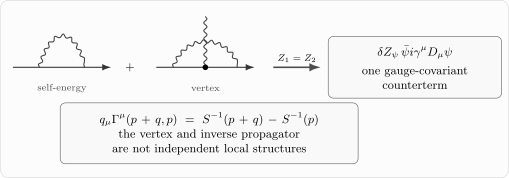
Gauge invariance does not allow the derivative term and the photon-fermion vertex to renormalize as unrelated local structures. They combine into the covariant counterterm $\delta Z_\psi\bar\psi i\gamma^\mu D_\mu\psi$.

Similarly, the photon two-point function cannot generate a photon mass term

$$M_A^2 A_\mu A^\mu,$$

because this term is not gauge invariant. The leading gauge-invariant photon counterterm is instead

$$\delta\mathcal L_A=-{\delta Z_A\over4e^2}F_{\mu\nu}F^{\mu\nu},$$

or, in canonical normalization, $-\delta Z_A F_{\rm can}^2/4$. The momentum-space tensor structure of the two-point function is therefore transverse,

$$\Pi_{\mu\nu}(q)=\left(q_\mu q_\nu-q^2\eta_{\mu\nu}\right)\Pi(q^2),$$

up to local contact terms organized into the same structure. The next page computes this object explicitly and extracts the running of the electric charge.

The Pauli term and magnetic moments

The dimension-five Pauli operator is

$$\mathcal O_P=\bar\psi\sigma^{\mu\nu}\psi F_{\mu\nu}.$$

It is gauge invariant because $F_{\mu\nu}$ is gauge invariant and $\bar\psi\psi$-type bilinears are neutral. It is Lorentz invariant because the antisymmetric tensor indices are contracted. Its dimension is

$$[\bar\psi\sigma^{\mu\nu}\psi F_{\mu\nu}] ={3\over2}+{3\over2}+2=5,$$

so its coefficient has dimension $-1$.

With the $1/4$ included in the definition of $c_P$ above, canonical normalization gives

$$\Delta\mathcal L_P={c_P e\over4\Lambda}\,\bar\psi\sigma^{\mu\nu}\psi F^{\rm can}_{\mu\nu}.$$

The factor $1/4$ is conventional and could instead be absorbed into $c_P$; the same normalization must simply be used in matching and in observables. For a nonrelativistic charged fermion, this operator shifts the coefficient of $\boldsymbol\sigma\cdot\mathbf B$, and therefore shifts the magnetic moment. If the UV theory approximately preserves chiral symmetry, the Pauli term is more suppressed than dimension counting alone suggests: it flips chirality, so its coefficient must be proportional to a chirality-breaking parameter such as the fermion mass.

This is a useful EFT lesson. Symmetry can improve power counting. Dimensional analysis tells us the power of $\Lambda$; symmetry tells us which dimensionless coefficient is allowed to be small or zero.

Four-fermion operators and weak interactions

The next classic EFT operator is a four-fermion contact interaction:

$$\boxed{ \Delta\mathcal L_4 ={c_4\over\Lambda^2}(\bar\psi\Gamma_1\psi)(\bar\chi\Gamma_2\chi). }$$

Each fermion has dimension $3/2$, so the operator has dimension $6$. It is irrelevant at low energies, but it can dominate when no dimension-four interaction connects the relevant particles.

The historical example is Fermi’s theory of beta decay. At energies much smaller than the $W$-boson mass, the weak decay

$$n\to p+e^-+\bar\nu_e$$

is described by a local current-current interaction,

$$\mathcal L_F =-{G_F\over\sqrt2} \left(\bar p\gamma^\mu(1-g_A\gamma^5)n\right) \left(\bar e\gamma_\mu(1-\gamma^5)\nu_e\right)+\cdots.$$

The coefficient has dimension $-2$:

$$[G_F]=-2.$$

In the Standard Model, this local term is the low-energy limit of $W$ exchange. Schematically,

$${g^2\over M_W^2-q^2} ={g^2\over M_W^2}\left(1+{q^2\over M_W^2}+\cdots\right), \qquad q^2\ll M_W^2.$$

The leading term gives the Fermi interaction, while the higher powers of $q^2/M_W^2$ generate higher-derivative operators.

The standard numerical matching follows once the current normalization is fixed. Write the charged-current interaction as

$$\mathcal L_{\rm cc} =-{g\over2\sqrt2} \left(W^+_\mu j_-^\mu+W^-_\mu j_+^\mu\right),$$

where $j_\pm^\mu$ are written with $(1-\gamma^5)$ rather than the projector $P_L=(1-\gamma^5)/2$. Tree-level $W$ exchange then gives

$$\mathcal L_{\rm eff} =-{g^2\over8M_W^2}j_+^\mu j_{-\mu} +O\left({g^2\over M_W^4}j_+^\mu\partial^2j_{-\mu}\right).$$

Comparing with $-G_Fj_+\cdot j_-/\sqrt2$ yields

$$\boxed{{G_F\over\sqrt2}={g^2\over8M_W^2}.}$$

Different factors quoted for this relation almost always come from using $P_L$ currents in one formula and $(1-\gamma^5)$ currents in another.

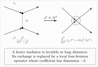
At momenta much smaller than the heavy mediator mass $M$, exchange of the heavy field collapses to a local four-fermion interaction. The expansion parameter is $q^2/M^2$.

This example is worth holding onto. It shows why nonrenormalizable operators are not a sign of failure. They are the low-energy footprints of particles or dynamics that have been integrated out.

Scalar QED and gauge completion

A charged scalar field makes a useful warning about gauge invariance. Its leading Lagrangian is

$$\mathcal L_{\mathrm{scalar\ QED}} =-{1\over4e^2}F_{\mu\nu}F^{\mu\nu} +(D_\mu\phi)^*(D^\mu\phi)-m^2\phi^*\phi-\lambda(\phi^*\phi)^2.$$

Expanding the covariant derivative gives

$$(D_\mu\phi)^*(D^\mu\phi) =(\partial_\mu\phi)^*(\partial^\mu\phi) -iA_\mu\left(\phi\partial^\mu\phi^*-\phi^*\partial^\mu\phi\right) +A_\mu A^\mu\phi^*\phi.$$

The last term is the seagull interaction. It is not optional. It is part of the same gauge-invariant operator as the scalar kinetic term.

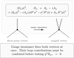
The scalar kinetic operator $|D_\mu\phi|^2$ generates both the one-photon derivative vertex and the two-photon seagull vertex. Gauge invariance fixes their relative coefficients.

This matters for loop calculations. In scalar QED, the photon vacuum polarization receives contributions from diagrams with two derivative vertices and from the seagull vertex. Individual diagrams may look non-transverse, but the gauge-invariant sum satisfies

$$q^\mu\Pi_{\mu\nu}(q)=0.$$

The moral is general: an EFT operator should be expanded only after the gauge-invariant structure has been identified. The diagrams are components of the operator, not independent physical assumptions.

Field redefinitions and operator bases

The list of allowed operators is not unique. Operators that differ by integration by parts, Bianchi identities, algebraic identities, or the leading equations of motion may give the same on-shell physics. For example, in the rescaled gauge-field normalization the leading Maxwell equation in the presence of the unit-charge current $J^\nu=\bar\psi\gamma^\nu\psi$ is schematically

$$\partial_\mu F^{\mu\nu}=-e^2 J^\nu.$$

Therefore an operator such as

$$(D_\mu F^{\mu\nu})(D^\rho F_{\rho\nu})$$

can often be traded, up to field redefinitions and higher-order effects, for current-current operators. This does not mean the operator is meaningless. It means that an EFT basis is a coordinate system on the space of local interactions, and different bases can describe the same observables.

A local field redefinition illustrates the point. Let

$$D\!\!\!/\equiv\gamma^\mu D_\mu.$$

A dimension-six redefinition such as

$$\psi\mapsto \psi+{a\over\Lambda^2}D^2\psi$$

changes the leading kinetic term by operators proportional to the Dirac equation,

$$(iD\!\!\!/-m)\psi=0,$$

plus higher-order local terms. Such changes move coefficients among operators but leave physical $S$-matrix elements unchanged. A good operator basis removes these redundancies so that the Wilson coefficients correspond to independent measurements rather than to a choice of field coordinates.

Integrating out the electron

So far the electron has remained a dynamical field. At energies much lower than the electron mass,

$$E\ll m_e,$$

one may integrate out the electron too. The EFT then contains photons only. The first terms after the Maxwell term are not all quartic in the field strength. A gauge-invariant derivative expansion also permits

$${c_6\over m_e^2}F_{\mu\nu}\Box F^{\mu\nu}.$$

For source-free on-shell photons this operator is redundant at the order shown: integration by parts and the leading Maxwell equation reduce it to an equation-of-motion term. It does, however, encode momentum-dependent two-point matching off shell or in the presence of currents. The first nontrivial on-shell photon interaction contains four field strengths and has dimension eight. In canonical photon normalization it is the Euler–Heisenberg operator,

$$\mathcal L_{\mathrm{EH}} ={\alpha^2\over90m_e^4} \left[ (F^{\rm can}_{\mu\nu}F_{\rm can}^{\mu\nu})^2 +{7\over4}(F^{\rm can}_{\mu\nu}\widetilde F_{\rm can}^{\mu\nu})^2 \right]+\cdots.$$

In terms of the canonically normalized electric and magnetic fields this is

$$\mathcal L_{\mathrm{EH}} ={2\alpha^2\over45m_e^4} \left[(\mathbf E^2-\mathbf B^2)^2+7(\mathbf E\cdot\mathbf B)^2\right]+\cdots.$$

This term describes low-energy light-by-light scattering. It is tiny at ordinary energies because it is suppressed by $m_e^{-4}$. But it is conceptually perfect: a loop of a particle that no longer appears as an external state becomes a local operator in the photon effective action.

Summary

QED is not just one Lagrangian. It is an organizing principle for a whole family of low-energy theories constrained by gauge invariance, Lorentz symmetry, locality, and the chosen light fields.

The renormalizable QED Lagrangian contains the leading relevant and marginal operators:

$$-{1\over4e^2}F^2+\bar\psi i\gamma^\mu D_\mu\psi-m\bar\psi\psi.$$

The Wilsonian EFT contains more:

$$\mathcal L_{\mathrm{eff}} =\mathcal L_{\mathrm{QED}} +{c_P\over4\Lambda}\bar\psi\sigma^{\mu\nu}\psi F_{\mu\nu} +{c_4\over\Lambda^2}(\bar\psi\Gamma\psi)^2 +{c_6\over\Lambda^2}F_{\mu\nu}\Box F^{\mu\nu} +{c_1\over\Lambda^4}(F^2)^2+\cdots.$$

The coefficients run with scale and mix under renormalization. Gauge invariance restricts which counterterms are allowed. In particular, vacuum polarization renormalizes $F^2$, not a photon mass. This is the conceptual setup for the next calculation.

Common pitfalls

Treating “nonrenormalizable” as a verdict. The word is a power-counting classification, not a claim that the operator is inconsistent. Higher-dimensional operators are expected and necessary in an effective theory.

Mixing photon normalizations. In canonical normalization, the photon kinetic term is $-F_{\rm can}^2/4$ and the charge appears in $D_\mu$. In the rescaled normalization used above, the unit-charge covariant derivative contains $A_\mu$ while the kinetic term is $-F^2/(4e^2)$; Wilson coefficients must be rescaled with the field.

Using power counting without symmetries. A photon mass is relevant by dimension but forbidden by gauge invariance. A Pauli term is dimension five but may require an additional chiral-symmetry-breaking insertion.

Keeping only part of a gauge completion. Expanding a gauge-invariant operator produces a linked set of vertices. In scalar QED, the derivative coupling and seagull coupling are tied together by $|D_\mu\phi|^2$, and dropping either one spoils the Ward identity.

Mistaking an operator list for a unique basis. Integration by parts, field redefinitions, and lowest-order equations of motion can move effects among higher-dimensional operators. Matching and running must therefore use one declared basis consistently.

Exercises

Exercise 1: Power count the leading QED EFT operators

Verify the engineering dimensions

$$[A_\mu]=1, \qquad [F_{\mu\nu}]=2, \qquad [\psi]={3\over2},$$

in four dimensions. Then find the dimensions of

$$\bar\psi\sigma^{\mu\nu}\psi F_{\mu\nu}, \qquad (\bar\psi\gamma^\mu\psi)(\bar\psi\gamma_\mu\psi), \qquad (F_{\mu\nu}F^{\mu\nu})^2.$$

Solution

The action is dimensionless and

$$S=\int d^4x\,\mathcal L,$$

so $[\mathcal L]=4$. From the Maxwell term,

$$F_{\mu\nu}F^{\mu\nu},$$

we get $2[F]=4$, hence

$$[F_{\mu\nu}]=2.$$

Since $F_{\mu\nu}=\partial_\mu A_\nu-\partial_\nu A_\mu$ and $[\partial]=1$,

$$[A_\mu]=1.$$

From the Dirac kinetic term,

$$\bar\psi i\gamma^\mu\partial_\mu\psi,$$

we find

$$[\bar\psi]+1+[\psi]=4.$$

Since $[\bar\psi]=[\psi]$,

$$[\psi]={3\over2}.$$

Therefore

$$[\bar\psi\sigma^{\mu\nu}\psi F_{\mu\nu}] =3+2=5,$$ $$[(\bar\psi\gamma^\mu\psi)(\bar\psi\gamma_\mu\psi)] =3+3=6,$$

and

$$[(F_{\mu\nu}F^{\mu\nu})^2]=4+4=8.$$

Their coefficients therefore scale as $1/\Lambda$, $1/\Lambda^2$, and $1/\Lambda^4$, respectively.

Exercise 2: Translate between the two photon normalizations

Start from canonical QED,

$$\mathcal L=-{1\over4}F_{\mu\nu}^{\mathrm{can}}F_{\mathrm{can}}^{\mu\nu} +\bar\psi\left(i\gamma^\mu(\partial_\mu-ieA^{\mathrm{can}}_\mu)-m\right)\psi.$$

Define $A_\mu=eA_\mu^{\mathrm{can}}$. Show that the Lagrangian becomes

$$\mathcal L=-{1\over4e^2}F_{\mu\nu}(A)F^{\mu\nu}(A) +\bar\psi\left(i\gamma^\mu(\partial_\mu-iA_\mu)-m\right)\psi.$$

Solution

Since

$$A_\mu=eA_\mu^{\mathrm{can}},$$

we have

$$F_{\mu\nu}(A)=\partial_\mu A_\nu-\partial_\nu A_\mu =e(\partial_\mu A_\nu^{\mathrm{can}}-\partial_\nu A_\mu^{\mathrm{can}}) =eF_{\mu\nu}^{\mathrm{can}}.$$

Thus

$$F_{\mu\nu}^{\mathrm{can}}F_{\mathrm{can}}^{\mu\nu} ={1\over e^2}F_{\mu\nu}(A)F^{\mu\nu}(A),$$

so the photon kinetic term becomes

$$-{1\over4}F_{\mathrm{can}}^2=-{1\over4e^2}F(A)^2.$$

The covariant derivative term transforms as

$$\partial_\mu-ieA_\mu^{\mathrm{can}}=\partial_\mu-iA_\mu.$$

Putting these together gives the desired Lagrangian.

Exercise 3: Derive transversality from the Ward identity

Assume Lorentz invariance gives

$$\Pi_{\mu\nu}(q)=A(q^2)\eta_{\mu\nu}+B(q^2)q_\mu q_\nu.$$

Use the Ward identity $q^\mu\Pi_{\mu\nu}(q)=0$ to show that

$$\Pi_{\mu\nu}(q)=\left(q_\mu q_\nu-q^2\eta_{\mu\nu}\right)\Pi(q^2).$$

Explain why this forbids a photon mass counterterm.

Solution

Contracting with $q^\mu$ gives

$$q^\mu\Pi_{\mu\nu}(q) =\left(A(q^2)+q^2B(q^2)\right)q_\nu.$$

The Ward identity requires

$$A(q^2)+q^2B(q^2)=0,$$

so

$$A(q^2)=-q^2B(q^2).$$

Therefore

$$\Pi_{\mu\nu}(q)=B(q^2)(q_\mu q_\nu-q^2\eta_{\mu\nu}).$$

Renaming $B(q^2)=\Pi(q^2)$ gives the stated form.

A photon mass counterterm would be proportional to $A_\mu A^\mu$, which contributes to the two-point function as a term proportional to $\eta_{\mu\nu}$ with a nonzero value at $q=0$. But the transverse structure above vanishes at $q=0$ up to the tensor factor $q_\mu q_\nu-q^2\eta_{\mu\nu}$. The allowed local counterterm is therefore $F_{\mu\nu}F^{\mu\nu}$, not $A_\mu A^\mu$.

Exercise 4: Integrate out a heavy vector at tree level

A heavy vector field $W_\mu$ of mass $M$ couples to a conserved current $J^\mu$ as

$$\mathcal L\supset {1\over2}M^2W_\mu W^\mu+gW_\mu J^\mu,$$

where derivatives of $W_\mu$ are neglected because the process has $q^2\ll M^2$. Eliminate $W_\mu$ using its algebraic equation of motion and find the leading current-current operator.

Solution

The equation of motion for $W_\mu$ is

$$M^2W_\mu+gJ_\mu=0,$$

so

$$W_\mu=-{g\over M^2}J_\mu.$$

Substituting back,

$${1\over2}M^2W_\mu W^\mu+gW_\mu J^\mu ={1\over2}M^2{g^2\over M^4}J_\mu J^\mu -{g^2\over M^2}J_\mu J^\mu.$$

Hence

$$\Delta\mathcal L_{\mathrm{eff}} =-{g^2\over2M^2}J_\mu J^\mu.$$

The overall sign depends on metric and on how the massive-vector quadratic term is written, but the EFT scaling is invariant:

$$\Delta\mathcal L_{\mathrm{eff}}\sim {g^2\over M^2}J_\mu J^\mu.$$

This is a dimension-six operator suppressed by $M^2$.

Exercise 5: Recover the scalar-QED seagull interaction

For scalar QED with

$$D_\mu\phi=(\partial_\mu-iA_\mu)\phi,$$

expand $(D_\mu\phi)^*(D^\mu\phi)$ and identify the one-photon and two-photon interactions.

Solution

We have

$$(D_\mu\phi)^*=\partial_\mu\phi^*+iA_\mu\phi^*.$$

Therefore

$$(D_\mu\phi)^*(D^\mu\phi) =(\partial_\mu\phi^*+iA_\mu\phi^*) (\partial^\mu\phi-iA^\mu\phi).$$

Multiplying out,

$$(D_\mu\phi)^*(D^\mu\phi) =\partial_\mu\phi^*\partial^\mu\phi -iA^\mu\phi\partial_\mu\phi^* +iA_\mu\phi^*\partial^\mu\phi +A_\mu A^\mu\phi^*\phi.$$

Equivalently,

$$(D_\mu\phi)^*(D^\mu\phi) =|\partial_\mu\phi|^2 -iA_\mu(\phi\partial^\mu\phi^*-\phi^*\partial^\mu\phi) +A_\mu A^\mu|\phi|^2.$$

The term linear in $A_\mu$ gives the one-photon scalar vertex. The term quadratic in $A_\mu$ gives the two-photon seagull vertex. Gauge invariance fixes both terms together.

References

• Thomas Appelquist and J. Carazzone, “Infrared Singularities and Massive Fields”, Physical Review D 11 (1975) 2856–2861.
• Enrico Fermi, “Versuch einer Theorie der $\beta$-Strahlen. I,” Zeitschrift für Physik 88 (1934) 161–177.
• Werner Heisenberg and Hans Euler, “Folgerungen aus der Diracschen Theorie des Positrons”, Zeitschrift für Physik 98 (1936) 714–732.
• Steven Weinberg, “Phenomenological Lagrangians”, Physica A 96 (1979) 327–340.

Further reading

• Aneesh V. Manohar, “Effective Field Theories”, in Perturbative and Nonperturbative Aspects of Quantum Field Theory, Lecture Notes in Physics 479, Springer (1997) 311–362.
• Matthew D. Schwartz, Quantum Field Theory and the Standard Model, Cambridge University Press (2014), Chapters 21–23, 33, and 34.
• Mark Srednicki, Quantum Field Theory, Cambridge University Press (2007), Sections 28–29 and 58–66.
• Steven Weinberg, The Quantum Theory of Fields, Vol. I: Foundations, Cambridge University Press (1995), Chapters 11–12; Vol. II: Modern Applications, Cambridge University Press (1996), Chapter 18.
• A. Zee, Quantum Field Theory in a Nutshell, 2nd ed., Princeton University Press (2010), Parts III and VIII.