

Conformal Transformations in d Dimensions
At a continuum RG fixed point, correlation functions of scaling operators become scale covariant. When the stress-tensor criterion of Lesson 13 holds, the spacetime symmetry extends to conformal symmetry: transformations that may stretch lengths by a position-dependent factor, but preserve angles. We assume that extension here and study its kinematic consequences at separated points.
We derive the conformal Killing equation, explain why two dimensions are exceptional, classify the generators in , and construct inversion and special conformal transformations. A connected special-conformal Ward identity then forces scalar-primary two-point functions of unequal dimensions to vanish. Inversion provides an alternative check when it is also a symmetry of the theory. The next page develops three- and four-point functions and the operator product expansion.
Required background. Lesson 13 derives fixed-point scaling and explains the stress-tensor criterion that promotes scale symmetry to conformal symmetry.
Helpful background. Lesson 12 supplies the scaling-dimension and Ising-operator conventions used in the correlator examples.
Conformal maps as local similarities
Section titled “Conformal maps as local similarities”A differentiable map is conformal when its Jacobian is locally a scale times an orthogonal matrix:
Equivalently,
or in components,
A circle of tangent vectors is therefore mapped to a circle by the derivative. A right angle remains a right angle, while every tangent-vector length is multiplied by . For a nonlinear map this statement describes the infinitesimal limit; a finite circle need not remain a circle. The figure illustrates the derivative itself.
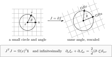
The quantitative illustration applies to a tangent circle of radius and unit vectors , . Both panels use the same coordinate scale. Every radius and vector length grows by , while the angle between the vectors is unchanged. This is a linear tangent map, not a claim about finite neighborhoods of an arbitrary nonlinear map.
An isometry is the special case . A dilation with has . Unit-sphere inversion has a nonconstant scale factor, away from the origin; its role as geometry must be distinguished from its possible role as a quantum symmetry.
Infinitesimal form: the conformal Killing equation
Section titled “Infinitesimal form: the conformal Killing equation”Let
Then
so, to first order in ,
A conformal transformation may only change the metric by a scalar factor. Hence
Taking the trace gives
and therefore
This is the conformal Killing equation. Ordinary Killing vectors obey the same equation with the right-hand side set to zero. Conformal Killing vectors are allowed to have a trace part; that trace is the infinitesimal local scale transformation.
The elementary solutions are
The special conformal vector is worth checking once. Differentiating gives
so it indeed satisfies the conformal Killing equation.
Two dimensions: holomorphic freedom
Section titled “Two dimensions: holomorphic freedom”In two Euclidean dimensions write
For , the conformal Killing equation becomes
These are precisely the Cauchy–Riemann equations, so
The antiholomorphic component satisfies
Thus the local conformal transformations are
with holomorphic and antiholomorphic functions, at least locally where the derivatives do not vanish. For a real orientation-preserving map of the Euclidean plane, the two functions are complex conjugates. In the complexified conformal algebra they are treated as independent left- and right-moving sectors.
The word “local” matters. On the Riemann sphere, the globally nonsingular one-to-one orientation-preserving conformal maps are only the Möbius transformations
On a punctured coordinate patch, local holomorphic vector fields have a Laurent basis,
which obey
The quantum version of this algebra, after central extension, will become the Virasoro algebra.
The finite group for d greater than two
Section titled “The finite group for d greater than two”For , the conformal Killing equation is much more rigid. Differentiating and permuting indices gives
Take of this identity and use . This gives
Its trace gives . For the Hessian of therefore vanishes: is affine, and the displayed second-derivative identity makes at most quadratic on a connected smooth patch. The general solution is
Counting parameters gives
For , the Lie algebra of Euclidean conformal transformations is
Equivalently, the identity component of the conformal group is locally isomorphic to . Global statements require the conformal compactification and a discrete quotient; inversion lies outside the identity component.
A useful differential-operator basis is
With these sign conventions,
The finite-dimensional algebra for should be compared with the infinite-dimensional local algebra in . That contrast is one of the central structural facts of conformal field theory.
Inversion and special conformal transformations
Section titled “Inversion and special conformal transformations”Inversion in the unit sphere, on the patch , is
Its Jacobian is
The matrix in parentheses reflects the radial direction and fixes the transverse directions. Its determinant is , so inversion is outside the identity component. It is nevertheless a useful geometric construction, whether or not the quantum theory has this additional discrete symmetry. See Rychkov 2016, arXiv v2, §2.2.1, p. 25, and §2.3.3, p. 31, PDF. Orthogonality gives
Thus inversion has local scale factor
For two points,
we find
Equivalently,
The figure checks the endpoint factors on an explicit pair of points.
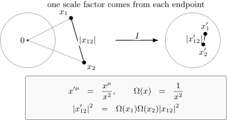
The quantitative unit-sphere inversion uses and in dimensionless coordinates, giving and . Both panels use the same scale. Each endpoint has , so the separation changes from to and its square by . This is a geometric identity; no inversion symmetry of a quantum theory is assumed.
A special conformal coordinate map can be constructed by inversion, followed by translation, followed by inversion. With the convention
one obtains
For , the denominator equals , so the finite Euclidean chart excludes . The origin has a regular image despite the intermediate inversions. The map belongs to the connected conformal group on the compactification; using two inversions to construct it does not require either inversion to be a quantum symmetry. Expanding to first order in gives
which is exactly the infinitesimal special conformal vector.
Primary scalar fields and two-point functions
Section titled “Primary scalar fields and two-point functions”Assume a conformally invariant vacuum and scalar primaries that diagonalize dilations. For connected conformal transformations, a primary of dimension has the local transformation law
If inversion is also a symmetry and is inversion-even without operator mixing, the same law reads
At separated insertions, the corresponding covariance law for connected conformal maps is
For a scalar two-point function of identical primaries,
the distance identity gives an algebraic inversion-covariance check:
For spinning primaries one must also rotate the indices by the local orthogonal matrix
For connected maps this local matrix is a proper rotation. Its representation on tensor or spinor indices is essential for spinning primaries. An extension to reflections requires additional discrete-symmetry data.
Now consider two scalar primaries of dimensions and . Translation, rotation, and scale invariance allow
Connected special-conformal symmetry supplies the stronger constraint. Expanding the covariance law with and gives the Ward identity
Use translation invariance to set and . The second insertion contributes zero. Writing , the radial form gives and . Consequently
For arbitrary nonzero separation this requires equal dimensions or a vanishing coefficient:
This proof requires no inversion symmetry. An embedding-space derivation and the scalar covariance formulas are given in Rychkov 2016, arXiv v2, §2.2.1, pp. 24–26, PDF. Contact terms at coincident points are outside the argument.
If several scalar primaries share a dimension and compatible internal quantum numbers, their two-point coefficients form a constant matrix. For Hermitian operators in a unitary theory one can diagonalize the positive two-point form after removing null operators. For complex operators the positive form pairs each operator with its adjoint. None of this makes two different equal-dimension operators identical.
Relation to the Ising fields
Section titled “Relation to the Ising fields”In the two-dimensional critical Ising theory, the identity , spin field , disorder field , and energy field can all be represented as scalar conformal fields. Their dimensions are
These dimensions are developed in Di Francesco, Mathieu and Sénéchal 1997, §§12.2.1–12.2.2, pp. 443–445 and translated to this course’s conventions in Lesson 12. Conformal covariance therefore predicts
It also predicts, in a basis adapted to conformal symmetry, that
because . The equality is consistent with Kramers–Wannier duality, but it does not mean that and are the same local operator. They are mutually nonlocal: taking an order field around a disorder field detects a branch cut. In the diagonal local Ising CFT, one chooses a mutually local operator algebra rather than treating both lattice realizations as independent local primaries. Conformal invariance fixes powers and tensor structures; the operator algebra still remembers the order–disorder construction.
Summary
Section titled “Summary”Conformal symmetry is the symmetry of local angle preservation. Its infinitesimal form is the conformal Killing equation
In two dimensions this equation becomes the Cauchy–Riemann equation, producing infinitely many local conformal maps. In it has only the finite-dimensional solution space generated by translations, rotations, dilations, and special conformal transformations.
Inversion is the key finite transformation. Its distance identity
provides a geometric covariance check. The scalar selection rule follows from a connected special-conformal Ward identity; treating inversion as a quantum symmetry is an additional assumption.
Common pitfalls
Section titled “Common pitfalls”The factor multiplies lengths, not squared lengths. The metric transforms with .
The statement that two-dimensional conformal maps are arbitrary holomorphic functions is local. Globally regular maps on the sphere are Möbius transformations.
For a real Euclidean conformal map, the antiholomorphic function is the complex conjugate of the holomorphic one. Treating the two sectors as independent refers to the complexified algebra.
Inversion is singular at the origin and exchanges the origin with infinity. It lies outside the identity component; a conformal theory need not be invariant under it. Algebraic inversion identities are usually cleanest on the conformal compactification.
For , the conformal group is locally related to , but the exact global group depends on connected components and a discrete quotient. The Lie-algebra statement refers to this finite-dimensional case, not the full local algebra in two dimensions.
Scale invariance alone permits a two-point function proportional to . The condition comes from the larger conformal group.
The Library treatment of Conformal Geometry, Maps, and Compactification develops the domain and global-extension questions behind these local formulas. It is the continuation for deciding whether a transformation remains defined across an inversion singularity or compactification patch.
Exercises
Section titled “Exercises”Exercise 1: Special conformal Killing vector
Section titled “Exercise 1: Special conformal Killing vector”Verify that
satisfies the conformal Killing equation.
Solution
Differentiate:
Therefore
The divergence is
Thus
which matches the symmetrized derivative.
Exercise 2: Cauchy–Riemann equations
Section titled “Exercise 2: Cauchy–Riemann equations”Show that the two-dimensional conformal Killing equation is equivalent to the Cauchy–Riemann equations for .
Solution
For ,
The component gives
so
The component gives
These are exactly the Cauchy–Riemann equations, so .
Exercise 3: Inversion of a separation
Section titled “Exercise 3: Inversion of a separation”Derive the inversion distance formula
Solution
Compute directly:
Exercise 4: Equal dimensions from inversion covariance
Section titled “Exercise 4: Equal dimensions from inversion covariance”Assume in addition that inversion preserves the vacuum and that the two scalar primaries are inversion-even with no mixing. Use inversion covariance to recover the equal-dimension condition already derived above from connected symmetry. Take separated points away from the inversion origin.
Solution
Start from the scale-invariant form
At inverted points this becomes
Primary covariance gives instead
If , the powers of and must match independently, so
Thus . If the dimensions differ, .
Exercise 5: Infinitesimal special conformal transformation
Section titled “Exercise 5: Infinitesimal special conformal transformation”Show that
has infinitesimal form
Solution
Expand the denominator:
Then
so
Subtracting gives the result.
References
Section titled “References”- Di Francesco, Philippe, Pierre Mathieu, and David Sénéchal. Conformal Field Theory. Springer, 1997. DOI.
- Rychkov, Slava. EPFL Lectures on Conformal Field Theory in D ≥ 3 Dimensions. arXiv:1601.05000v2 (2016). Versioned PDF. Locators above refer to the preprint’s printed pages.
Further reading
Section titled “Further reading”- Cardy, John. Scaling and Renormalization in Statistical Physics. Cambridge University Press, 1996. DOI.