Callan–Symanzik Equations and Marginal Operators

The previous page described the Wilsonian RG as a change of resolution: integrate out a thin shell of high-momentum modes, then rewrite the result as a new local action. That viewpoint is physical and constructive, but in perturbative QFT we often use a slightly different language. We introduce a subtraction scale $\mu$ when defining renormalized couplings and fields. That scale is arbitrary. A physical correlation function cannot depend on where we chose to subtract.

The Callan–Symanzik equation is the differential expression of this arbitrariness. It says that explicit dependence on the subtraction scale is cancelled by implicit dependence through running couplings, masses, and operator normalizations. In this form, the RG becomes a first-order partial differential equation for correlation functions.

The main conceptual bridge is:

$$\text{Wilsonian flow of effective actions} \quad\Longleftrightarrow\quad \text{Callan–Symanzik flow of renormalized correlators}.$$

The first describes how the Lagrangian changes when the cutoff changes. The second describes how a fixed physical answer is represented in different renormalized coordinates. They are not competing stories. They are two coordinate systems on the same scale-dependence.

Required background. Wilsonian RG and operator mixing supplies the shell-integration law, the ultraviolet time $t=\log(k/\Lambda)$, and the operator-mixing equation used here. Helpful background. Operator product expansion in perturbation theory explains why the collision of two marginal interaction insertions produces the logarithm that becomes a beta function.

From shell composition to Callan–Symanzik transport

Scale variables used below. The global QFT II conventions are used. We write the renormalization scale as $\mu$ and define beta functions at fixed bare parameters:

$$\beta_i(\vec g)=\mu {\partial g_i\over\partial\mu}\bigg|_{\rm bare}.$$

For a one-component scalar field,

$$\phi_0=Z_\phi^{1/2}\phi, \qquad \gamma_\phi={1\over2}\mu {\partial\log Z_\phi\over\partial\mu}\bigg|_{\rm bare}.$$

With this definition, connected renormalized $n$-point functions obey a Callan–Symanzik equation with $+n\gamma_\phi$, while one-particle-irreducible $n$-point vertices obey the corresponding equation with $-n\gamma_\phi$. This sign difference is only a consequence of whether external field factors appear in the numerator or denominator.

The differential equation first appears before any field-renormalization factors are introduced. Let $\mathcal Z(\vec g,k)$ denote a generating functional, or any dimensionless renormalized quantity, written using couplings $\vec g$ at a reference momentum $k$. Performing a short RG step and then another must give the same result as performing the combined step. Consequently there are running couplings $\bar g_i(s;\vec g)$ such that

$$\mathcal Z(\vec g,k) =\mathcal Z\bigl(\bar{\vec g}(s;\vec g),sk\bigr), \qquad \bar{\vec g}(1;\vec g)=\vec g.$$

This composition law is the shortest route from finite changes of resolution to a differential equation. Differentiating at $s=1$ gives

$$\boxed{ \left( {\partial\over\partial\log k} +\sum_i\beta_i(\vec g){\partial\over\partial g_i} \right)\mathcal Z(\vec g,k)=0, }$$

where

$$\beta_i(\vec g) =\left.{\partial\bar g_i(s;\vec g)\over\partial\log s}\right|_{s=1}.$$

Equivalently,

$${\partial\mathcal Z\over\partial\log k} =-\sum_i\beta_i{\partial\mathcal Z\over\partial g_i}.$$

This is the compact Callan–Symanzik formula. The symbol used for the running reference scale is immaterial; we call it $k$ here so it is not confused with a fixed ultraviolet regulator $\Lambda$. When $k$ and the subtraction scale $\mu$ both increase toward the ultraviolet, their beta-function signs agree. With the infrared coarse-graining time $L=\log(k_0/k)$, every flow acquires the opposite sign.

The characteristic equations are now immediate:

$${d\log k\over dt}=1, \qquad {d\bar g_i\over dt}=\beta_i(\bar{\vec g}), \qquad {d\mathcal Z\over dt}=0.$$

Thus the RG equation does not say that the physics changes with the arbitrary scale. It says that the coordinates used to describe the same physics move along a beta-function trajectory. Correlators with elementary or composite insertions obey the same transport law, supplemented by the anomalous-dimension terms derived next.

Renormalized correlators and bare independence

What is fixed when differentiating?

The phrase “differentiate at fixed bare parameters” is a bookkeeping device, not a physical experiment. It means that the same regulated path integral is being described with a different subtraction scale $\mu$. The bare symbols $g_0,m_0,\Lambda$ are held fixed while the renormalized coordinates $g(\mu)$ and $m(\mu)$ change. Physical observables do not change; their representation in renormalized variables does.

This is why the Callan–Symanzik equation has two kinds of terms. The explicit $\mu\partial_\mu$ term differentiates logarithms left in a correlator, while the $\beta_i\partial_{g_i}$ and anomalous-dimension terms differentiate the running parameters and operator normalizations used to write the same correlator.

Start with a regularized theory. The regulator can be a hard cutoff $\Lambda$, dimensional regularization, a lattice spacing, Pauli–Villars fields, or something else. The details matter for intermediate formulas, but not for the structural point.

Let

$$G_0^{(n)}(x_1,\ldots,x_n;g_0,m_0,\Lambda) =\langle\phi_0(x_1)\cdots\phi_0(x_n)\rangle$$

be a bare connected correlation function. The renormalized field is defined by

$$\phi_0=Z_\phi^{1/2}(\vec g,\mu,\Lambda)\,\phi,$$

so the corresponding renormalized connected correlator is

$$G_R^{(n)}(x_1,\ldots,x_n;\vec g,m,\mu) =Z_\phi^{-n/2}G_0^{(n)}(x_1,\ldots,x_n;g_0,m_0,\Lambda).$$

The bare parameters $g_0,m_0$ are not independent of the renormalized parameters $\vec g,m,\mu$. They are chosen so that a specified set of renormalization conditions is satisfied. Schematically,

$$g_0=g_0(\vec g,m,\mu,\Lambda), \qquad m_0=m_0(\vec g,m,\mu,\Lambda).$$

Now comes the crucial observation: the bare correlator has no reason to know about the arbitrary subtraction scale $\mu$. The symbol $\mu$ was introduced by us when we defined renormalized coordinates. Therefore

$$\mu {d\over d\mu}G_0^{(n)}\bigg|_{g_0,m_0,\Lambda}=0.$$

Using

$$G_0^{(n)}=Z_\phi^{n/2}G_R^{(n)},$$

and differentiating at fixed bare parameters gives

$$0=\mu {d\over d\mu}\left(Z_\phi^{n/2}G_R^{(n)}\right)_{\rm bare}.$$

The derivative acts in three ways: on explicit $\mu$ dependence, on renormalized couplings and masses, and on the field normalization $Z_\phi$. Define

$$\beta_i(\vec g)=\mu {\partial g_i\over\partial\mu}\bigg|_{\rm bare}, \qquad \beta_m(\vec g,m)=\mu {\partial m\over\partial\mu}\bigg|_{\rm bare},$$

and

$$\gamma_\phi(\vec g)={1\over2}\mu {\partial\log Z_\phi\over\partial\mu}\bigg|_{\rm bare}.$$

Then

$$\boxed{ \left( \mu {\partial\over\partial\mu} +\sum_i\beta_i(\vec g){\partial\over\partial g_i} +\beta_m(\vec g,m){\partial\over\partial m} +n\gamma_\phi(\vec g) \right)G_R^{(n)}=0. }$$

This is the Callan–Symanzik equation for connected field correlators. Some authors write the mass term as $\gamma_m m\partial_m$ or use $m^2\partial_{m^2}$ instead. These are equivalent after specifying whether the running variable is $m$ or $m^2$; what matters is that the relevant mass deformation is transported together with the dimensionless couplings.

For one-particle-irreducible vertices $\Gamma_R^{(n)}$, the external field normalization appears oppositely. Since

$$\Gamma_R^{(n)}=Z_\phi^{n/2}\Gamma_0^{(n)},$$

the corresponding equation is

$$\boxed{ \left( \mu {\partial\over\partial\mu} +\sum_i\beta_i(\vec g){\partial\over\partial g_i} +\beta_m(\vec g,m){\partial\over\partial m} -n\gamma_\phi(\vec g) \right)\Gamma_R^{(n)}=0. }$$

At one loop in four-dimensional $\phi^4$ theory, $\gamma_\phi$ begins only at two loops, so the sign of the field-anomalous-dimension term is invisible in the simplest four-point calculation. It becomes essential in general.

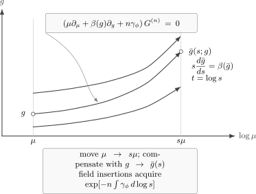
The Callan–Symanzik equation says that changing the arbitrary subtraction scale $\mu$ can be compensated by moving along the running coupling $g(\mu)$. Correlators are transported along these characteristic curves, with field-renormalization factors governed by anomalous dimensions.

The equation as a cancellation of logarithms

The simplest way to see the equation at work is to revisit the four-point vertex in massless four-dimensional scalar theory. Use the Euclidean interaction

$$S_{\rm int}=\int d^4x\,{\lambda\over4!}\phi^4.$$

At a symmetric Euclidean subtraction point of momentum scale $\mu$, define

$$\lambda\equiv \Gamma_4(\mu).$$

The one-loop leading-log result at another scale $q$ has the form

$$\Gamma_4(q;\lambda,\mu) =\lambda-a\lambda^2\log {\mu\over q}+O(\lambda^3), \qquad a={3\over16\pi^2}.$$

The explicit $\mu$ derivative gives

$$\mu{\partial\Gamma_4\over\partial\mu} =-a\lambda^2+O(\lambda^3).$$

The beta function is

$$\beta(\lambda)=a\lambda^2+O(\lambda^3).$$

Therefore, through order $\lambda^2$,

$$\left(\mu{\partial\over\partial\mu}+\beta(\lambda){\partial\over\partial\lambda}\right) \Gamma_4(q;\lambda,\mu) = -a\lambda^2+a\lambda^2+O(\lambda^3)=0.$$

The logarithm is not a nuisance added to the theory. It is precisely the visible trace of the running coupling. The arbitrary scale $\mu$ enters the fixed-order formula explicitly, but the coupling defined at $\mu$ changes in exactly the way needed to keep the physical vertex invariant.

This cancellation is the local version of the Wilsonian statement from the previous page. There, lowering a cutoff shell shifted the coupling. Here, changing the subtraction point shifts the renormalized coupling. In both descriptions, the coefficient of the logarithm is the coefficient of the beta function.

Characteristics and RG improvement

The Callan–Symanzik equation is a first-order partial differential equation. Its natural solution is by characteristics.

For one dimensionless coupling and no mass, write the connected $n$-point equation as

$$\left( \mu {\partial\over\partial\mu} +\beta(g){\partial\over\partial g} +n\gamma_\phi(g) \right)G_R^{(n)}=0.$$

Define the running coupling $\bar g(s)$ by

$$s{d\bar g\over ds}=\beta(\bar g), \qquad \bar g(1)=g.$$

Along the curve

$$\mu\longrightarrow s\mu, \qquad g\longrightarrow \bar g(s),$$

the Callan–Symanzik equation becomes the ordinary differential equation

$$s{d\over ds}G_R^{(n)}(x_i;\bar g(s),s\mu) =-n\gamma_\phi(\bar g(s))G_R^{(n)}(x_i;\bar g(s),s\mu).$$

Hence

$$\boxed{ G_R^{(n)}(x_i;g,\mu) = \exp\left[ n\int_1^s {ds'\over s'}\gamma_\phi(\bar g(s')) \right] G_R^{(n)}(x_i;\bar g(s),s\mu). }$$

Equivalently, solving for the correlator at the transported point,

$$G_R^{(n)}(x_i;\bar g(s),s\mu) = \exp\left[ -n\int_1^s {ds'\over s'}\gamma_\phi(\bar g(s')) \right] G_R^{(n)}(x_i;g,\mu).$$

This formula is the analytic form of RG improvement. A fixed-order calculation often contains logarithms such as

$$\log {q\over\mu} \quad\text{or}\quad \log(\mu |x|).$$

If these logarithms are large, perturbation theory with a coupling defined at $\mu$ is poorly organized. The characteristic solution tells us to choose $s$ so that

$$s\mu\sim q \qquad\text{in momentum space},$$

or

$$s\mu\sim {1\over |x|} \qquad\text{in coordinate space}.$$

Then the large logarithms are moved into $\bar g(s)$ and the anomalous-dimension exponential. That is the practical meaning of “use the running coupling at the physical scale.”

For one-loop $\phi^4$ theory,

$$\mu {d\lambda\over d\mu}=a\lambda^2,$$

so

$${d\over d\log\mu}\left({1\over\lambda}\right)=-a.$$

Thus

$$\boxed{ {1\over\lambda(\mu_2)}={1\over\lambda(\mu_1)}-a\log{\mu_2\over\mu_1}. }$$

Equivalently,

$$\boxed{ \lambda(\mu_2) ={\lambda(\mu_1)\over1-a\lambda(\mu_1)\log(\mu_2/\mu_1)}. }$$

If $\mu_2<\mu_1$ and $\lambda>0$, the denominator is larger than one, so the coupling decreases in the infrared. If $\mu_2>\mu_1$, the coupling grows and eventually reaches the perturbative Landau pole

$$\mu_{\rm L}=\mu_1\exp\left({1\over a\lambda(\mu_1)}\right).$$

The pole is not a trustworthy prediction of strong coupling physics. It is a warning that the one-loop weak-coupling description cannot be extrapolated indefinitely.

Scaling at a fixed point

A fixed point is a point in coupling space where all beta functions vanish:

$$\beta_i(\vec g_*)=0.$$

At such a point, scale transformations no longer move the couplings. If the theory is massless and no relevant deformation is turned on, the Callan–Symanzik equation becomes a scaling equation.

For a scalar field, combine the Callan–Symanzik equation with ordinary dimensional analysis. The engineering dimension of a free scalar in $d$ Euclidean dimensions is

$$\Delta_\phi^{\rm cl}={d-2\over2}.$$

At a fixed point, the anomalous dimension is a number

$$\gamma_{\phi,*}=\gamma_\phi(\vec g_*),$$

and the full scaling dimension is

$$\boxed{ \Delta_\phi={d-2\over2}+\gamma_{\phi,*}. }$$

Therefore the fixed-point two-point function has the power-law form

$$\boxed{ \langle\phi(x)\phi(0)\rangle_* ={C_\phi\over |x|^{2\Delta_\phi}}. }$$

The constant $C_\phi$ depends on the normalization of $\phi$, but the exponent is physical once the scaling operator is normalized consistently.

For a composite operator $\mathcal O_A$, renormalization generally mixes all operators with the same quantum numbers. Write

$$\mathcal O_A^{(0)}=Z_A{}^B\mathcal O_B.$$

The anomalous-dimension matrix is

$$\gamma_A{}^B=(Z^{-1})_A{}^C\, \mu{\partial Z_C{}^B\over\partial\mu}\bigg|_{\rm bare}.$$

At a fixed point, diagonalizing

$$\Delta_A{}^B=\Delta_A^{\rm cl}\delta_A{}^B+\gamma_A{}^B$$

gives scaling operators. There is an index-ordering detail worth making explicit. With the convention

$$\mu {d\mathcal O_A\over d\mu}=-\gamma_A{}^B\mathcal O_B,$$

a linear combination $\widehat{\mathcal O}_a=v_a{}^A\mathcal O_A$ has definite anomalous dimension when $v_a{}^A$ is a left eigenvector,

$$v_a{}^A\gamma_A{}^B=\gamma_a v_a{}^B.$$

Equivalently, one may transpose every matrix and use right eigenvectors; physical scaling dimensions do not depend on this bookkeeping choice. If $\widehat{\mathcal O}_a$ has dimension $\Delta_a$, then

$$\boxed{ \langle\widehat{\mathcal O}_a(x)\widehat{\mathcal O}_a(0)\rangle_* \propto {1\over |x|^{2\Delta_a}}. }$$

This is the cleanest interpretation of anomalous dimensions: they are the quantum correction to the exponents of correlation functions at scale-invariant points.

What is invariant at a fixed point?

The entries of an anomalous-dimension matrix depend on the operator basis, but its eigenvalues at a fixed point are scaling dimensions and are physical data of the fixed point. Away from a fixed point, anomalous dimensions still control logarithms, but they are scheme- and basis-dependent functions rather than standalone observables.

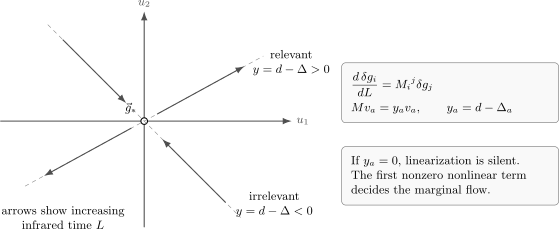
Near a fixed point, the beta-function vector field can be linearized. Eigen-directions with $\Delta<d$ are relevant and grow under infrared coarse graining; those with $\Delta>d$ are irrelevant and die away; marginal directions require higher-order beta-function terms.

Relevant, irrelevant, and marginal perturbations

Perturb a fixed point by local operators:

$$S=S_*+\sum_a u_a\mu^{d-\Delta_a}\int d^dx\,\mathcal O_a(x).$$

The $u_a$ are dimensionless couplings. To first order near the fixed point,

$$\boxed{ \mu {d u_a\over d\mu}=(\Delta_a-d)u_a+O(u^2). }$$

This is the Callan–Symanzik version of the Wilsonian operator hierarchy. If we instead use infrared RG time

$$L=\log{\mu_0\over\mu},$$

then

$$\boxed{ {d u_a\over dL}=(d-\Delta_a)u_a+O(u^2). }$$

Thus:

Operator type	Scaling dimension	Behavior under infrared coarse graining
relevant	$\Delta_a<d$	grows and must be tuned to reach the fixed point
irrelevant	$\Delta_a>d$	shrinks and is forgotten at long distances
marginal	$\Delta_a=d$	decided by nonlinear terms in the beta function

A mass term is the standard relevant deformation of a scalar fixed point. At the Gaussian fixed point in $d=4$,

$$\Delta_{\phi^2}=2,$$

so

$$S\supset {1\over2}m^2\int d^4x\,\phi^2$$

has coupling dimension $2$. The dimensionless ratio

$$r(\mu)={m^2(\mu)\over\mu^2}$$

therefore grows as $\mu$ is lowered. This is why the mass must be tuned to study critical behavior. By contrast, $\phi^6$ in four dimensions has $\Delta=6$ and is irrelevant at the Gaussian fixed point.

At an interacting fixed point, the same classification holds, but $\Delta_a$ includes anomalous dimensions. In critical phenomena, the leading relevant eigenvalue determines the correlation-length exponent. In high-energy language, the same mathematics describes how a renormalized mass or coupling departs from a scale-invariant theory.

Marginal operators and logarithmic fate

Marginal operators are delicate because dimensional analysis gives no linear verdict. Suppose $g$ couples to a marginal operator, so the beta function begins as

$$\beta(g)=b_2g^2+b_3g^3+\cdots.$$

The first nonzero coefficient decides the fate near $g=0$.

If $b_2>0$ and $g>0$, then

$$\mu {dg\over d\mu}=b_2g^2$$

implies that $g$ decreases toward the infrared. The perturbation is marginally irrelevant in the infrared. Four-dimensional scalar $\phi^4$ theory at positive weak coupling has exactly this behavior at one loop.

If $b_2<0$ and $g>0$, then $g$ grows toward the infrared and decreases toward the ultraviolet. The perturbation is marginally relevant in the infrared and asymptotically free in the ultraviolet. In gauge theory one often writes

$$\beta(g)=-b_0g^3+O(g^5), \qquad b_0>0,$$

because the gauge coupling $g$ rather than $g^2$ is used. In terms of $\alpha\propto g^2$, the leading beta function is quadratic:

$$\mu {d\alpha\over d\mu}=-B\alpha^2+O(\alpha^3).$$

If every coefficient vanishes along a family of theories,

$$\beta(g)=0,$$

then the operator is exactly marginal. Exactly marginal directions generate continuous families of fixed points. They are special; ordinary marginality by power counting is not enough.

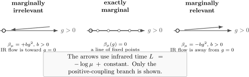
A classically marginal coupling has no linear RG term. Higher-order terms decide whether it is exactly marginal, marginally irrelevant in the infrared, or marginally relevant in the infrared. The arrows show infrared flow.

The logarithmic running of a marginal coupling is slower than the power-law running of relevant or irrelevant couplings. That slowness is why marginal operators dominate so many quantum-field-theoretic phenomena: Landau poles, asymptotic freedom, logarithmic corrections to scaling, Kosterlitz–Thouless-type flows, and dimensional transmutation all begin with marginality.

Example: the four-point vertex as a Callan–Symanzik problem

Return to the renormalized four-point vertex in massless $\phi^4$ theory. Define

$$\lambda=\Gamma_4(q=\mu).$$

The one-loop beta function is

$$\beta(\lambda)=a\lambda^2+O(\lambda^3), \qquad a={3\over16\pi^2}.$$

The one-loop RG-improved vertex is

$$\boxed{ \Gamma_4(q) ={\lambda(\mu)\over 1+a\lambda(\mu)\log(\mu/q)}. }$$

Check that it is independent of $\mu$ to the order controlled by the beta function. Differentiate the inverse form

$${1\over\Gamma_4(q)}={1\over\lambda(\mu)}+a\log{\mu\over q}.$$

At fixed $q$,

$$\mu{d\over d\mu}{1\over\Gamma_4(q)} =-{1\over\lambda^2}\beta(\lambda)+a =-a+a+O(\lambda)=0.$$

Thus the apparent $\mu$ dependence cancels. The same formula may be written as

$$\Gamma_4(q)=\lambda(q),$$

where $\lambda(q)$ is the running coupling obtained from $\lambda(\mu)$ by solving the beta-function equation down to scale $q$.

The small-coupling expansion is

$$\Gamma_4(q) =\lambda-a\lambda^2\log{\mu\over q} +a^2\lambda^3\log^2{\mu\over q} -\cdots.$$

The leading logarithms are not independent calculations. They are generated by repeatedly applying the same first-order Callan–Symanzik equation.

Composite insertions and operator mixing

The Callan–Symanzik equation becomes richer when correlation functions contain composite operators. Let

$$G_A^{(n)}(x;y_1,\ldots,y_n) =\langle\mathcal O_A(x)\phi(y_1)\cdots\phi(y_n)\rangle_R.$$

If the operators mix as

$$\mathcal O_A^{(0)}=Z_A{}^B\mathcal O_B,$$

then

$$\boxed{ \left( \mu {\partial\over\partial\mu} +\sum_i\beta_i{\partial\over\partial g_i} +\beta_m{\partial\over\partial m} +n\gamma_\phi \right)G_A^{(n)} + \gamma_A{}^B G_B^{(n)}=0. }$$

This formula is the Callan–Symanzik version of the operator-mixing discussion from the previous page. A basis of local operators is not generally preserved by renormalization. The operator labels rotate under changes of scale.

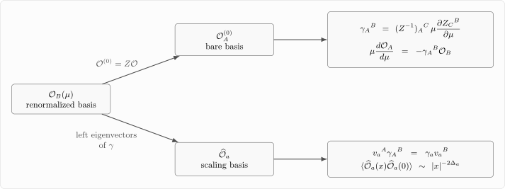
Composite operators with the same quantum numbers generally mix. The anomalous-dimension matrix $\gamma_A{}^B$ is diagonalized at a fixed point to obtain scaling operators with definite dimensions.

This is especially important for the operator product expansion. The OPE at a fixed point takes the schematic form

$$\mathcal O_A(x)\mathcal O_B(0) \sim \sum_C C_{AB}{}^C(x)\mathcal O_C(0),$$

where the coefficient functions scale as

$$C_{AB}{}^C(x)\propto {1\over |x|^{\Delta_A+\Delta_B-\Delta_C}}$$

up to tensor structures and normalization conventions. Away from a fixed point, these coefficient functions acquire logarithmic dependence controlled by the same beta functions and anomalous-dimension matrices.

The lesson is that anomalous dimensions are not optional decorations on operators. They are the data needed to say how local probes change when the microscope scale changes.

Scale Ward identity and the trace of the stress tensor

The Callan–Symanzik equation can also be read as a quantum scale Ward identity. Classically, a massless theory with dimensionless couplings may appear scale invariant. Quantum mechanically, the renormalization scale $\mu$ enters, and the beta functions measure the failure of scale invariance.

In a local QFT, an infinitesimal scale transformation is generated by the trace of the stress tensor. Schematically,

$$\boxed{ T^\mu{}_{\mu} = \sum_i\beta_i(\vec g)\,\mathcal O_i +\sum_a (d-\Delta_a)u_a\mu^{d-\Delta_a}\mathcal O_a +\text{equation-of-motion and improvement terms}. }$$

The first term is the anomalous breaking associated with marginal couplings. The second term is explicit breaking by relevant or irrelevant deformations. Equation-of-motion terms depend on the operator basis and vanish inside separated-point correlators of physical operators. Improvement terms reflect the freedom to redefine the stress tensor by total derivatives.

At a fixed point with all relevant deformations tuned away,

$$\beta_i(\vec g_*)=0,$$

and the trace can be set to zero in the improved stress tensor in the standard relativistic examples of interest here. That is why fixed points are the natural home of scaling dimensions, OPE coefficients, and universal correlation functions.

This viewpoint will reappear in several forms later: the two-dimensional models make scale and conformal ideas especially sharp; sigma models use beta functions to turn classical scale invariance into mass generation; Yang–Mills theory uses the trace anomaly to replace a dimensionless coupling by a physical scale.

Summary

The Callan–Symanzik equation follows from a simple fact: bare quantities do not depend on the arbitrary renormalization scale $\mu$. For connected renormalized $n$-point functions,

$$\left( \mu {\partial\over\partial\mu} +\sum_i\beta_i{\partial\over\partial g_i} +\beta_m{\partial\over\partial m} +n\gamma_\phi \right)G_R^{(n)}=0.$$

For 1PI vertices, the field-anomalous-dimension term has the opposite sign:

$$\left( \mu {\partial\over\partial\mu} +\sum_i\beta_i{\partial\over\partial g_i} +\beta_m{\partial\over\partial m} -n\gamma_\phi \right)\Gamma_R^{(n)}=0.$$

At a fixed point, anomalous dimensions correct engineering dimensions:

$$\Delta_\phi={d-2\over2}+\gamma_{\phi,*},$$

and composite operators must be diagonalized under the anomalous-dimension matrix to obtain scaling operators.

Perturbing a fixed point by

$$u_a\mu^{d-\Delta_a}\int\mathcal O_a$$

gives, to linear order,

$$\mu {du_a\over d\mu}=(\Delta_a-d)u_a.$$

Relevant perturbations have $\Delta_a<d$, irrelevant perturbations have $\Delta_a>d$, and marginal perturbations have $\Delta_a=d$. For marginal operators, nonlinear beta-function terms decide the fate: exactly marginal, marginally irrelevant, or marginally relevant.

The four-dimensional $\phi^4$ coupling is classically marginal, but at weak positive coupling

$$\beta(\lambda)={3\lambda^2\over16\pi^2}+O(\lambda^3),$$

so it is marginally irrelevant in the infrared and grows toward the ultraviolet.

Common pitfalls

Confusing the cutoff with the subtraction scale. A Wilsonian cutoff is the resolution of an effective action, whereas a subtraction scale labels renormalized coordinates. They can be varied in parallel, but they are not the same object.

Treating classical marginality as a final answer. Marginal means only that the linearized flow vanishes. The first nonzero nonlinear beta-function coefficient decides whether the perturbation is marginally relevant, marginally irrelevant, or exactly marginal.

Using one anomalous-dimension sign for every Green function. Connected $n$-point functions carry $+n\gamma_\phi$ in the convention used here, while 1PI vertices carry $-n\gamma_\phi$. The difference follows from the opposite external-field factors and should be rederived if a different $Z_\phi$ convention is adopted.

Diagonalizing the wrong matrix action. Composite operators with the same symmetries mix, and the side on which eigenvectors act depends on the index convention. With $\mu d\mathcal O_A/d\mu=-\gamma_A{}^B\mathcal O_B$, coefficients of scaling operators are left eigenvectors of $\gamma$.

Reading a one-loop Landau pole literally. The pole marks the point where the weak-coupling resummation ceases to be controlled. It does not determine the ultraviolet completion or prove that an exact observable is singular there.

Exercises

Exercise 1: Derive the connected two-point Callan–Symanzik equation

Let a renormalized connected two-point function be related to the bare one by

$$G_R^{(2)}=Z_\phi^{-1}G_0^{(2)}.$$

Using

$$\gamma_\phi={1\over2}\mu{\partial\log Z_\phi\over\partial\mu}\bigg|_{\rm bare},$$

derive the Callan–Symanzik equation for $G_R^{(2)}$ in a massless one-coupling theory.

Solution

The bare correlator is independent of the subtraction scale at fixed bare parameters:

$$\mu{dG_0^{(2)}\over d\mu}\bigg|_{\rm bare}=0.$$

Since

$$G_0^{(2)}=Z_\phi G_R^{(2)},$$

we differentiate:

$$0=\mu{d\over d\mu}\left(Z_\phi G_R^{(2)}\right)_{\rm bare}.$$

The derivative of $Z_\phi$ gives

$$\mu{dZ_\phi\over d\mu}=2\gamma_\phi Z_\phi.$$

The derivative of $G_R^{(2)}$ acts explicitly and through the running coupling:

$$\mu{dG_R^{(2)}\over d\mu} =\left(\mu{\partial\over\partial\mu}+\beta(g){\partial\over\partial g}\right)G_R^{(2)}.$$

Therefore

$$0=Z_\phi\left[ 2\gamma_\phi G_R^{(2)} +\left(\mu{\partial\over\partial\mu}+\beta(g){\partial\over\partial g}\right)G_R^{(2)} \right].$$

Dividing by $Z_\phi$ gives

$$\boxed{ \left( \mu{\partial\over\partial\mu} +\beta(g){\partial\over\partial g} +2\gamma_\phi \right)G_R^{(2)}=0. }$$

Exercise 2: Read the beta function from a one-loop logarithm

A one-loop four-point vertex has the form

$$\Gamma_4(q;\lambda,\mu)=\lambda-a\lambda^2\log{\mu\over q}+O(\lambda^3).$$

Use the Callan–Symanzik equation

$$\left(\mu{\partial\over\partial\mu}+\beta(\lambda){\partial\over\partial\lambda}\right)\Gamma_4=0$$

to determine $\beta(\lambda)$ to order $\lambda^2$.

Solution

Differentiate explicitly with respect to $\mu$:

$$\mu{\partial\Gamma_4\over\partial\mu} =-a\lambda^2+O(\lambda^3).$$

Also,

$${\partial\Gamma_4\over\partial\lambda} =1+O(\lambda).$$

Write

$$\beta(\lambda)=b\lambda^2+O(\lambda^3).$$

The Callan–Symanzik equation gives

$$-a\lambda^2+b\lambda^2+O(\lambda^3)=0.$$

Hence

$$\boxed{\beta(\lambda)=a\lambda^2+O(\lambda^3).}$$

For one real scalar field with interaction $\lambda\phi^4/4!$ in four dimensions,

$$a={3\over16\pi^2}.$$

Exercise 3: Solve a marginal one-loop flow

Solve the beta-function equation

$$\mu{dg\over d\mu}=b g^2$$

with initial value $g(\mu_0)=g_0$. For $b>0$ and $g_0>0$, decide whether the coupling is marginally relevant or marginally irrelevant in the infrared.

Solution

Write the equation as

$${dg\over g^2}=b{d\mu\over\mu}=b\,d\log\mu.$$

Integrating from $\mu_0$ to $\mu$ gives

$$-{1\over g(\mu)}+{1\over g_0}=b\log{\mu\over\mu_0}.$$

Therefore

$${1\over g(\mu)}={1\over g_0}-b\log{\mu\over\mu_0},$$

or

$$\boxed{ g(\mu)={g_0\over1-bg_0\log(\mu/\mu_0)}. }$$

For infrared flow, take $\mu<\mu_0$. Then

$$\log{\mu\over\mu_0}<0,$$

so the denominator is larger than one. Thus $g(\mu)<g_0$. The coupling decreases in the infrared, so it is marginally irrelevant for $b>0$ and positive weak coupling.

Exercise 4: Diagonalize a composite-operator mixing matrix

At a fixed point, two operators $\mathcal O_1$ and $\mathcal O_2$ have the same engineering dimension $\Delta_0$ and obey

$$\mu{d\mathcal O_A\over d\mu}=-\gamma_A{}^B\mathcal O_B,$$

with anomalous-dimension matrix

$$\gamma= \begin{pmatrix} \gamma_1 & a\\ 0 & \gamma_2 \end{pmatrix}.$$

Assume $\gamma_1\neq\gamma_2$. Find linear combinations with definite dimensions. Pay attention to whether operator coefficients are left or right eigenvectors.

Solution

The full dimension matrix is

$$\Delta=\Delta_0 I+\gamma.$$

The eigenvalues are

$$\Delta_+=\Delta_0+\gamma_1, \qquad \Delta_- =\Delta_0+\gamma_2.$$

Because the operator RG equation is written as

$$\mu{d\mathcal O_A\over d\mu}=-\gamma_A{}^B\mathcal O_B,$$

the coefficients $v^A$ in $\widehat{\mathcal O}=v^A\mathcal O_A$ must form a left eigenvector:

$$v^A\gamma_A{}^B=\gamma_{\widehat{\mathcal O}}v^B.$$

For eigenvalue $\gamma_1$, write $v=(x,y)$. Then

$$(x,y) \begin{pmatrix} \gamma_1 & a\\ 0 & \gamma_2 \end{pmatrix} =\gamma_1(x,y),$$

which gives

$$xa=(\gamma_1-\gamma_2)y.$$

Taking $x=1$ gives

$$\boxed{ \widehat{\mathcal O}_1 =\mathcal O_1+{a\over\gamma_1-\gamma_2}\mathcal O_2, \qquad \Delta_1=\Delta_0+\gamma_1. }$$

For eigenvalue $\gamma_2$, the left-eigenvector equation forces $x=0$, so

$$\boxed{ \widehat{\mathcal O}_2=\mathcal O_2, \qquad \Delta_2=\Delta_0+\gamma_2. }$$

A quick check is to differentiate the two combinations directly: neither derivative contains the other operator. Right eigenvectors would be appropriate had we written the mixing equation with the transposed matrix acting on a column of operator coefficients.

Exercise 5: Convert fixed-point scaling into infrared flow

Let $u$ be a dimensionless coupling to an operator of scaling dimension $\Delta$ near a fixed point in $d$ dimensions:

$$S=S_*+u\mu^{d-\Delta}\int d^dx\,\mathcal O(x).$$

Show that the linearized beta function is

$$\beta_u=(\Delta-d)u.$$

Then rewrite the flow in infrared time $L=\log(\mu_0/\mu)$.

Solution

The dimensionful coefficient of $\int\mathcal O$ is

$$g_{\rm dimful}=u\mu^{d-\Delta}.$$

At the fixed point, the dimensionful coefficient should be independent of the arbitrary reference scale if only engineering scaling is considered:

$$0=\mu{d\over d\mu}\left(u\mu^{d-\Delta}\right).$$

This gives

$$0=\mu^{d-\Delta}\left(\mu{du\over d\mu}+(d-\Delta)u\right),$$

so

$$\boxed{ \mu{du\over d\mu}=(\Delta-d)u. }$$

Since

$$L=\log{\mu_0\over\mu}, \qquad {d\over dL}=-\mu{d\over d\mu},$$

we get

$$\boxed{ {du\over dL}=(d-\Delta)u. }$$

Thus $u$ grows in the infrared if $\Delta<d$, shrinks if $\Delta>d$, and requires nonlinear terms if $\Delta=d$.

References

• Curtis G. Callan Jr., “Broken Scale Invariance in Scalar Field Theory”, Physical Review D 2 (1970) 1541–1547.
• Kurt Symanzik, “Small Distance Behaviour in Field Theory and Power Counting”, Communications in Mathematical Physics 18 (1970) 227–246.
• Kenneth G. Wilson and J. Kogut, “The Renormalization Group and the ε Expansion”, Physics Reports 12 (1974) 75–200.

Further reading

• Matthew D. Schwartz, Quantum Field Theory and the Standard Model, Cambridge University Press (2014), Chapter 23.
• Mark Srednicki, Quantum Field Theory, Cambridge University Press (2007), Sections 27–29.
• Steven Weinberg, The Quantum Theory of Fields, Vol. II: Modern Applications, Cambridge University Press (1996), Chapter 18.
• Jean Zinn-Justin, Quantum Field Theory and Critical Phenomena, 4th ed., Oxford University Press (2002), Chapters 8–13.