

Causality, Commutators, and Support
The previous pages used the exact two-point function to identify particles: a physical particle appears as a pole, and the self-energy moves that pole away from the bare mass. This page turns from the momentum-space picture to the spacetime picture. Relativistic QFT must also answer a sharper question: how can a theory with quantum fluctuations everywhere avoid faster-than-light signaling?
The answer is not that all correlators vanish outside the light cone. They do not. The Feynman propagator is generally nonzero at spacelike separation. The causal statement is instead that commutators of local observables vanish at spacelike separation. For a scalar field, the basic form is
This property is called microcausality or local commutativity. It is one of the places where the field viewpoint is much cleaner than a single-particle relativistic wavefunction: locality is stated directly in spacetime, as an algebraic property of operators.
A useful way to keep the logic straight is this:
| Object | What it measures | Support property |
|---|---|---|
| vacuum fluctuations and positive-frequency propagation | generally nonzero at spacelike separation | |
| the kernel used inside perturbation theory | generally nonzero at spacelike separation | |
| whether two local operations can fail to commute | zero at spacelike separation | |
| causal response to a disturbance at | supported in the future light cone |
The vanishing statement is therefore not about correlations being absent. The vacuum can be correlated across spacelike separation. The statement is about controllable influence: no local operation at can change a measurement at a spacelike-separated point .
Equal-time algebra
Section titled “Equal-time algebra”This lesson preserves the course’s mode-expansion route to microcausality. Retarded, Advanced, and Spectral Correlators develops the commutator support, source signs, pole prescriptions, and the translation among common response-function conventions.
For a free real scalar field,
with
the standard mode expansion is
where
At equal time, direct substitution gives
The commutator vanishes because the integrand is odd under . The mixed commutator is instead
Thus the field is local in the canonical sense: at a fixed time, the field at one point only fails to commute with its conjugate momentum at the same point. Relativistic causality is the Lorentz-covariant extension of this statement.
The Pauli–Jordan commutator function
Section titled “The Pauli–Jordan commutator function”At unequal times, the same mode expansion gives
Changing in the second term yields
Therefore
where
The free Pauli–Jordan distribution satisfies the homogeneous Klein–Gordon equation everywhere in the distributional sense:
Its initial data are the canonical commutation relations:
The unequal-time commutator is therefore the relativistic propagation of the equal-time canonical algebra. The mode expansion, its antisymmetric frequency combination, and the causal support are developed in Schwartz 2014, § 12.6, pp. 220–221.
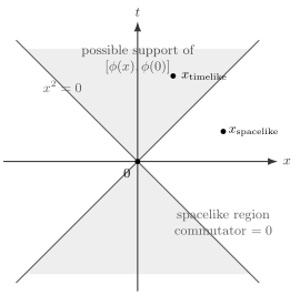
The scalar-field commutator has no support in the spacelike region. It may be nonzero inside or on the light cone, where causal propagation is possible.
A manifestly Lorentz-invariant form is
This formula makes it clear that depends only on Lorentz-invariant data: and, for timelike , the sign of .
The invariant form is also a good diagnostic for signs. Differentiating the equal-time expression gives , so is the retarded Green function with a positive delta-function source. If your convention defines , all signs in this paragraph reverse, but the light-cone support does not.
Vanishing outside the light cone
Section titled “Vanishing outside the light cone”There is a very efficient proof of microcausality. Suppose is spacelike:
Then some Lorentz frame makes the two events simultaneous. In that frame,
so the equal-time commutator gives
Because a scalar-field commutator transforms covariantly, an operator equality established in one inertial frame holds in every inertial frame. The boost argument does not require the commutator to be a c-number (although the free-field commutator constructed above is one). Hence
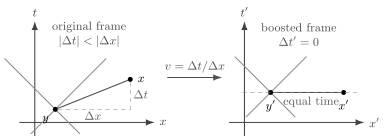
For spacelike separation, along the separation direction. A boost with makes the two events simultaneous, where the equal-time commutator vanishes.
Explicitly, for a separation along one spatial direction,
Choosing
is allowed because for spacelike separation, and it gives .
This is not just a trick for the free field. In any local relativistic QFT, microscopic causality is imposed as the condition that local observables commute at spacelike separation. It is what prevents two observers, who may disagree about the time ordering of spacelike separated events, from disagreeing about measurable physics.
Feynman propagation is not causal response
Section titled “Feynman propagation is not causal response”The Feynman propagator is
At fixed spatial momentum,
This expression carries positive-frequency modes forward in time and negative-frequency modes backward in time. It is the correct kernel for vacuum perturbation theory, but it is not the kernel for causal signal propagation.
For the free field, the retarded Green function is built from the c-number commutator:
It obeys
and has support only in the future light cone. The advanced response has support only in the past light cone. In an interacting theory, the commutator is generally operator-valued; linear response in a chosen state uses . Microcausality still fixes its support, but it no longer obeys the free Klein–Gordon equation displayed above.
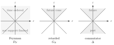
The Feynman propagator is a time-ordered vacuum correlator and is generally nonzero outside the light cone. The retarded response is built from the commutator and is supported only in the future light cone. The commutator has support in the union of the future and past light cones.
The distinction can be summarized by writing the Wightman function
Then
while the vacuum expectation value of the commutator is
The same two vacuum correlation functions appear in both expressions, but they are combined differently. Their time-ordered sum gives the Feynman propagator; their antisymmetric difference gives the expectation value of the causal commutator. For the free scalar, that commutator is a c-number, so it equals its vacuum expectation value.
Contact terms from time ordering
Section titled “Contact terms from time ordering”Time ordering is made of step functions. Derivatives of time-ordered products therefore produce delta functions. For two bosonic operators and ,
Differentiating gives
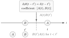
The derivative of the step function inside a time-ordered product gives a delta function. The coefficient of that delta function is the equal-time commutator.
For the scalar propagator, this contact term is exactly what makes a Green function of the Klein–Gordon operator:
with the sign following from the convention
The delta function is not a new physical interaction. It is the distributional imprint of the canonical commutator .
Local interactions and Lorentz-invariant perturbation theory
Section titled “Local interactions and Lorentz-invariant perturbation theory”For a local scalar interaction,
the interacting time-ordered correlator is expanded as
This formula seems to depend on a chosen time coordinate, because orders operators by time. The dependence is harmless only because spacelike separated local operators commute. If and are spacelike separated, different inertial observers may disagree about their order, but
Thus changing the order of spacelike separated interaction insertions changes nothing. Timelike orderings are invariantly ordered, and spacelike orderings are algebraically irrelevant. This is the spacetime reason why local perturbation theory can be Lorentz invariant.
There is a small but important qualification. For charged fields or gauge-variant fields, the field operator itself may not be a directly measurable local observable. The operational causality statement is about local gauge-invariant observables and local operator algebras. In the free scalar theory considered here, is already a local observable, so the commutator calculation displays the whole mechanism without extra gauge-theory complications.
Summary
Section titled “Summary”The equal-time canonical algebra evolves into the Pauli–Jordan commutator
where vanishes for spacelike separations. This is microcausality. It does not mean that all two-point functions vanish outside the light cone; it means that the part of a correlator capable of changing the order of local operations vanishes there.
The Feynman propagator is a time-ordered vacuum correlator, designed for perturbation theory. The retarded propagator is the causal response function, built from the commutator. Derivatives of time-ordered products produce contact terms, and those contact terms are required by the same equal-time algebra that enforces locality.
Common pitfalls
Section titled “Common pitfalls”- Confusing with a signal. The Feynman propagator can be nonzero at spacelike separation. Causality is governed by commutators and retarded functions.
- Forgetting that spacelike time ordering is frame dependent. Local commutativity is what makes different time orderings agree for spacelike-separated insertions.
- Dropping contact terms. Differentiating a time-ordered product differentiates the step functions. The resulting delta functions are essential.
- Mixing sign conventions. If you change the definition of or the metric signature, the signs in the Green-function equations change, but the support properties do not.
- Assuming equal-time commutators are enough. They are initial data. The full relativistic statement is the vanishing of local commutators for every spacelike separation.
- Forgetting the observable/operator distinction. In scalar theory itself is local. In gauge theory the same causality idea applies most directly to gauge-invariant local observables.
Exercises
Section titled “Exercises”Exercise 1
Section titled “Exercise 1”Starting from the scalar mode expansion, derive
Then verify .
Solution
Only the commutators contribute. Therefore
Changing in the second term gives
which is the desired expression. Differentiating with respect to gives
At this becomes
Exercise 2
Section titled “Exercise 2”Let two events have separation and along one spatial direction, with . Find a boost that makes them simultaneous, and use it to prove the vanishing of the scalar commutator for this separation.
Solution
Under a boost along the -direction,
Choose
Because the separation is spacelike, . Then . In that frame the canonical equal-time commutator gives
The scalar commutator is a Lorentz-covariant c-number distribution, so if it vanishes in one inertial frame for a given separation, it vanishes in all inertial frames. Hence
Exercise 3
Section titled “Exercise 3”Show that the retarded function
has support only for and, using microcausality, only inside or on the future light cone.
Solution
The factor makes for . For , we have
Microcausality says that this commutator vanishes whenever . Therefore can be nonzero only when both
and
This is precisely the future light cone, including its boundary.
Exercise 4
Section titled “Exercise 4”Prove the identity
for bosonic operators.
Solution
Start from
Differentiating gives
Since , the delta terms combine into
The remaining terms are exactly .
References
Section titled “References”- Schwartz, Matthew D. Quantum Field Theory and the Standard Model. Cambridge University Press, 2014, § 12.6, pp. 220–221. DOI.
Further reading
Section titled “Further reading”- Coleman, Sidney. Lectures of Sidney Coleman on Quantum Field Theory. Edited by Bryan Gin-ge Chen, David Derbes, David Griffiths, Brian Hill, Richard Sohn, and Yuan-Sen Ting. World Scientific, 2019. DOI.
- Peskin, Michael E., and Daniel V. Schroeder. An Introduction to Quantum Field Theory. Addison-Wesley, 1995, chapter 2. Publisher.
- Srednicki, Mark. Quantum Field Theory. Cambridge University Press, 2007. DOI.
- Weinberg, Steven. The Quantum Theory of Fields. Volume I: Foundations. Cambridge University Press, 1995. DOI.