Statistical Mechanics and Field Theory

The previous page converted the oscillatory Lorentzian weight $e^{iS}$ into the Euclidean weight $e^{-S_E}$. This is more than a technical trick. It is the point at which quantum field theory begins to look like statistical mechanics.

A Euclidean path integral sums over field configurations with a positive weight, at least for stable bosonic theories. A statistical-mechanical partition function also sums over configurations with a positive Boltzmann weight. Once those two statements are put next to each other, the basic dictionary is almost forced on us: the Euclidean action plays the role of an energy functional, sources play the role of external fields, and Euclidean correlation functions become ordinary statistical correlations.

This page develops that dictionary in the simplest setting. We start from the Ising model, pass to a coarse-grained order parameter, and obtain the Landau–Ginzburg field theory whose Gaussian correlator has the same form as a Euclidean scalar propagator. This is the doorway to the next page: near a critical point, the correlation length diverges, the effective mass goes to zero, and the long-distance behavior becomes universal.

Euclidean path integrals as statistical weights

Classical temperature versus Euclidean period

Throughout this page $k_B=1$, so inverse temperature is

$$\beta={1\over T}.$$

It is useful to distinguish two related but different statements. A $d$-dimensional Euclidean QFT can be read as a classical statistical field theory in $d$ dimensions. A finite-temperature quantum theory in $D$ spatial dimensions becomes a Euclidean path integral on $S^1_\beta\times \mathbb R^D$, with Euclidean time compactified to circumference $\beta$. The second statement will become central in the finite-temperature pages.

For a real scalar field in Euclidean signature, the generating functional is

$$Z_E[J] =\int \mathcal D\phi\,\exp\left[-S_E[\phi]+\int d^dx\,J(x)\phi(x)\right].$$

For the free theory,

$$S_{E,0}[\phi] ={1\over2}\int d^dx\,\phi(x)K_E\phi(x), \qquad K_E=-\partial^2+m^2.$$

The corresponding two-point function is the inverse of $K_E$:

$$\langle \phi(x)\phi(y)\rangle =K_E^{-1}(x,y),$$

or in momentum space,

$$\langle \phi(k)\phi(-k)\rangle ={1\over k^2+m^2}.$$

This is exactly the form one expects from a Gaussian statistical ensemble. If a variable $q$ has probability density proportional to $e^{-aq^2/2}$, then $\langle q^2\rangle=1/a$. A free Euclidean field is the infinite-dimensional version of that statement: each Fourier mode is a Gaussian variable, and the stiffness of mode $k$ is $k^2+m^2$.

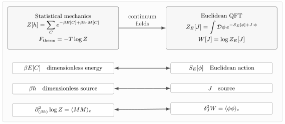
A Euclidean path integral has the structure of a statistical partition function. The Euclidean action $S_E$ replaces the dimensionless free-energy functional $\mathcal F=\beta F$, the field $\phi$ replaces an order parameter, and the Euclidean source corresponds to the dimensionless statistical source: $J\leftrightarrow\beta h_{\rm phys}$. Consequently the physical susceptibility is $\chi_{\rm phys}=\beta\langle MM\rangle_c$.

In classical statistical mechanics, a system with configurations $C$ and energy $E[C]$ has partition function

$$Z=\sum_C e^{-\beta E[C]}.$$

If $C$ is a continuous field configuration $m(x)$, this becomes formally

$$Z=\int \mathcal Dm\,e^{-\beta F[m]}.$$

Thus the Euclidean QFT expression and the statistical expression match after identifying

$$S_E[\phi]\quad \longleftrightarrow\quad \beta F[m].$$

One can either keep $F$ as a physical free energy and write $e^{-\beta F}$, or absorb the factor of $\beta$ into a dimensionless functional

$$\mathcal F[m]=\beta F[m], \qquad Z=\int \mathcal Dm\,e^{-\mathcal F[m]}.$$

Below we usually use the dimensionless functional $\mathcal F$ because it makes the formulas look identical to Euclidean QFT.

The Ising model and its sources

The simplest microscopic model with a nontrivial order parameter is the Ising model. Put a spin

$$\sigma_i=\pm1$$

at each site $i$ of a lattice. For a ferromagnet with nearest-neighbor coupling $J>0$ and external physical magnetic field $h_i$, the Hamiltonian is

$$H[\sigma] =-J\sum_{\langle ij\rangle}\sigma_i\sigma_j -\sum_i h_i\sigma_i.$$

The partition function is

$$Z[h] =\sum_{\{\sigma_i=\pm1\}}\exp\left[\beta J\sum_{\langle ij\rangle}\sigma_i\sigma_j +\beta\sum_i h_i\sigma_i\right].$$

This has precisely the same logic as a source functional. Differentiating with respect to $h_i$ inserts spins:

$$\langle \sigma_i\rangle ={1\over \beta}{\partial \log Z[h]\over \partial h_i},$$

and

$$\langle \sigma_i\sigma_j\rangle_c ={1\over \beta^2} {\partial^2 \log Z[h]\over \partial h_i\partial h_j}.$$

The logarithm selects connected correlations, just as $W[J]=\log Z[J]$ does in the QFT generating functional. The response of the magnetization to a small magnetic field is therefore a two-point function. For a uniform field, define the total magnetization

$$M=\sum_i \sigma_i.$$

Then the physical magnetic susceptibility is

$$\chi_{\rm phys} ={\partial \langle M\rangle\over \partial h}\bigg|_{h=0} =\beta\left(\langle M^2\rangle-\langle M\rangle^2\right).$$

This formula is a clean statistical-mechanical version of a lesson we have already seen in QFT: fluctuations and response are the same object viewed from two sides.

From lattice spins to an order-parameter field

A lattice spin $\sigma_i$ is not a smooth field. It jumps between $+1$ and $-1$ from site to site. But near a continuous phase transition, the important fluctuations are not individual spin flips. The important fluctuations are large correlated domains.

Choose blocks of linear size $\ell$ much larger than the microscopic lattice spacing $a$, but still much smaller than the macroscopic correlation length $\xi$:

$$a\ll \ell\ll \xi.$$

Define a coarse-grained magnetization field $m(x)$ by averaging spins in a block centered near $x$:

$$m(x) ={1\over N_\ell}\sum_{i\in \text{block}(x)}\sigma_i.$$

This field changes slowly on the scale of the lattice. Its precise microscopic definition is not unique, but long-distance physics should not depend on the details of the averaging procedure. That is the first glimpse of universality.

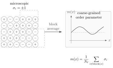
The Ising model has microscopic variables $\sigma_i=\pm1$. Coarse graining over blocks produces a smooth order-parameter field $m(x)$, whose long-wavelength fluctuations are described by a local functional $\mathcal F[m]$.

Once we describe the system by $m(x)$, the most general local functional compatible with the symmetries begins as a gradient expansion:

$$\mathcal F[m] =\int d^dx\left[ {\kappa\over2}(\nabla m)^2 +{r\over2}m^2 +{u\over4}m^4 -hm +\cdots \right].$$

Here $d$ is the number of spatial dimensions of the classical statistical system. The ellipsis denotes higher powers such as $m^6$, higher derivatives such as $(\nabla^2m)^2$, and terms with more fields and derivatives. The coefficients depend on microscopic physics and on temperature.

Because $\mathcal F$ is dimensionless, the source denoted by $h$ in this continuum functional is already the dimensionless source. If $h_{\rm phys}$ is the magnetic field appearing in a Hamiltonian, then schematically $h=\beta h_{\rm phys}$, with additional coarse-graining factors depending on the normalization of $m$.

It is therefore useful to name the source-normalized continuum response separately:

$$\chi_h\equiv {\partial\langle m\rangle\over\partial h} =G_m(k=0).$$

If the coarse-grained field has the same normalization as the physical magnetization density, then $\chi_{\rm phys}=\beta\chi_h$; a rescaling of $m$ supplies the corresponding field-normalization factors. The critical exponents are unchanged, but these factors matter for amplitudes.

The structure of this functional is not guessed randomly. The $\mathbb Z_2$ spin-flip symmetry $\sigma_i\mapsto -\sigma_i$ becomes $m(x)\mapsto -m(x)$ when $h=0$, so odd powers of $m$ are absent at zero field. Short-range microscopic interactions imply locality at long distance, so the functional can be expanded in powers of $m$ and its derivatives. Stability requires $u>0$ at this order, while $\kappa>0$ penalizes rapid spatial variation.

The normalization of the order-parameter field is not physical. If $\kappa$ is positive, one may define a canonically normalized field

$$\phi=\sqrt{\kappa}\,m.$$

Then the quadratic part becomes

$${1\over2}\int d^dx\left[(\nabla\phi)^2+{r\over\kappa}\phi^2\right],$$

and the quartic coupling is rescaled by powers of $\kappa$. The invariant statement is not the numerical value of $r$ or $u$ separately, but the long-distance correlation length, scaling behavior, and symmetry class.

The quadratic coefficient $r$ is the most important parameter near the transition. In mean-field theory,

$$r=a_0(T-T_c), \qquad a_0>0.$$

Thus $r>0$ above the critical temperature and $r<0$ below it.

Mean-field minima

For a uniform configuration and zero external field, the Landau potential is

$$V_L(m)={r\over2}m^2+{u\over4}m^4.$$

The stationary points obey

$${dV_L\over dm}=rm+um^3=m(r+um^2)=0.$$

If $r>0$, the only real minimum is

$$m=0.$$

This is the disordered phase. The average magnetization vanishes, and the $\mathbb Z_2$ symmetry is unbroken.

If $r<0$, the point $m=0$ becomes unstable and two degenerate minima appear:

$$m=\pm \sqrt{-{r\over u}}.$$

This is the ordered phase. The microscopic Hamiltonian still has the spin-flip symmetry, but an infinite system can choose one of the two minima. The order parameter distinguishes the phases.

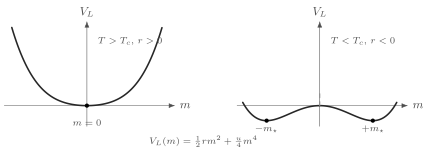
The Landau potential $V_L(m)=rm^2/2+um^4/4$ has a single minimum at $m=0$ when $r>0$, and two symmetry-related minima when $r<0$. The sign change of $r$ is the mean-field signal of the transition.

The critical point is where $r=0$. At this point the quadratic restoring force vanishes, long-wavelength fluctuations become cheap, and the correlation length diverges in the Gaussian approximation.

Gaussian fluctuations and correlation length

Above the critical temperature, the mean field is $m=0$. Keeping only the quadratic part of $\mathcal F$ gives

$$\mathcal F_2[m] ={1\over2}\int d^dx\left[\kappa(\nabla m)^2+r m^2\right].$$

Use the Fourier transform

$$m(x)=\int {d^dk\over(2\pi)^d}\,e^{ik\cdot x}m(k).$$

Then

$$\mathcal F_2[m] ={1\over2}\int {d^dk\over(2\pi)^d} (\kappa k^2+r)m(k)m(-k).$$

Define the momentum-space two-point kernel by stripping off the momentum-conserving delta function,

$$\langle m(k)m(k')\rangle =(2\pi)^d\delta^{(d)}(k+k')\,G_m(k).$$

The Gaussian rule immediately gives

$$\boxed{ G_m(k) ={1\over \kappa k^2+r} ={1\over\kappa}\,{1\over k^2+\xi^{-2}}. }$$

The correlation length is

$$\boxed{ \xi=\sqrt{\kappa\over r}. }$$

Thus $r$ is the statistical-mechanical analogue of the Euclidean mass squared. In QFT language,

$$m_{\mathrm{eff}}^2={r\over\kappa}, \qquad \xi={1\over m_{\mathrm{eff}}}.$$

This is the central bridge of the page: a massive Euclidean propagator describes short-range correlations, and a massless Euclidean propagator describes scale-free critical fluctuations.

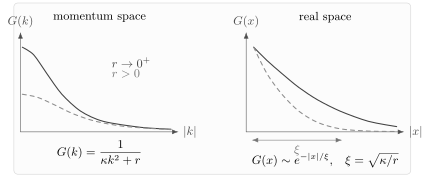
The Gaussian order-parameter correlator is $G(k)=1/(\kappa k^2+r)$. As $r\to0^+$, the correlation length $\xi=\sqrt{\kappa/r}$ diverges and long-wavelength fluctuations dominate.

In three dimensions, the real-space correlator is explicitly

$$G(x)=\langle m(x)m(0)\rangle ={1\over \kappa}\int {d^3k\over(2\pi)^3}\,{e^{ik\cdot x}\over k^2+\xi^{-2}} ={1\over4\pi\kappa |x|}e^{-|x|/\xi}.$$

The field theory has converted a thermodynamic question into the study of Green functions. The pole at

$$k^2=-\xi^{-2}$$

controls the exponential decay of correlations. The same statement, analytically continued, is the QFT statement that poles determine particle propagation.

Free energy, connected diagrams, and why log Z matters

The partition function itself is usually not the final observable. The free energy is

$$F_{\mathrm{therm}}=-T\log Z.$$

This is why $\log Z$ is the natural object. In a source-dependent ensemble,

$$W[h]=\log Z[h]$$

generates connected spin correlators. In a Euclidean QFT,

$$W[J]=\log Z[J]$$

generates connected field correlators. Perturbatively, this means that disconnected vacuum pieces exponentiate, and the logarithm of the partition function receives only connected vacuum diagrams.

This is not a minor bookkeeping convenience. In statistical mechanics, the free energy is extensive:

$$F_{\mathrm{therm}}\propto \text{volume}.$$

Disconnected diagrams would overcount independent pieces of the system. Connected diagrams are the contributions that cannot be decomposed into independent subsystems. The same connected/disconnected distinction that organized Feynman diagrams now becomes the statement that thermodynamic potentials are additive over distant regions.

Why φ⁴ theory appears

The Landau–Ginzburg functional for an Ising-like system has the same long-distance structure as Euclidean $\phi^4$ theory:

$$S_E[\phi] =\int d^dx\left[ {1\over2}(\nabla\phi)^2 +{1\over2}m_0^2\phi^2 +{\lambda\over4!}\phi^4 \right].$$

Using the canonically normalized field $\phi=\sqrt\kappa\,m$, the precise correspondence in the conventions above is

$$m_0^2={r\over\kappa}, \qquad \lambda={6u\over\kappa^2}, \qquad J={h\over\sqrt\kappa}.$$

If one starts instead from the physical magnetic field in the Boltzmann factor, the last relation reads $J=\beta h_{\rm phys}/\sqrt\kappa$. These normalization factors do not affect the symmetry class or universal long-distance behavior, but they matter when comparing formulas coefficient by coefficient.

The reason this works is that the long-distance theory is constrained mainly by symmetry and locality. For the Ising universality class, the order parameter is a single real scalar and the symmetry is $\phi\mapsto-\phi$. The first nontrivial stable interaction is therefore $\phi^4$.

This also explains why the exact lattice details are not expected to matter near a continuous transition. A square lattice, a cubic lattice, and many short-range microscopic Hamiltonians can flow to the same continuum field theory because their differences appear as higher-order operators that are less important at long distances. This claim will become sharper once renormalization enters the story.

Summary

Euclidean QFT and statistical mechanics share the same mathematical skeleton. Both compute weighted sums over configurations. Both generate correlations by differentiating with respect to sources. Both organize connected observables through $\log Z$.

The Ising model gives the cleanest physical example. Microscopic spins $\sigma_i=\pm1$ can be coarse-grained into an order-parameter field $m(x)$. Symmetry and locality then lead to the Landau–Ginzburg functional

$$\mathcal F[m] =\int d^dx\left[ {\kappa\over2}(\nabla m)^2+{r\over2}m^2+{u\over4}m^4-hm+\cdots\right].$$

After removing the overall momentum-conserving delta function, the Gaussian correlator is

$$G_m(k)={1\over \kappa k^2+r},$$

so the correlation length is

$$\xi=\sqrt{\kappa\over r}.$$

The effective mass of the Euclidean field is the inverse correlation length. A critical point is therefore a massless limit of a Euclidean field theory. This is the conceptual engine behind the relation between QFT, critical phenomena, and the renormalization group.

Common pitfalls

A Euclidean path integral is not automatically a probability measure. The analogy with statistical mechanics is cleanest for stable bosonic Euclidean actions. Gauge fields require gauge fixing, fermions require Grassmann variables, and sign problems can appear in more general systems.

The parameter called “mass” in the Euclidean statistical field theory is not always a microscopic particle mass. In this context, $m_{\mathrm{eff}}=\xi^{-1}$ is an inverse correlation length. It becomes a particle mass only after the appropriate analytic continuation and physical interpretation.

Mean-field theory is not exact near a critical point in low dimensions. The Landau functional is an excellent starting point, but fluctuations modify critical exponents below the upper critical dimension. The next page begins to show how loop corrections detect this failure.

Do not assign physical meaning to the normalization of $m(x)$ itself. A rescaling of the coarse-grained field changes $\kappa$, $r$, and $u$, but it cannot change the correlation length $\xi$ or universal critical exponents.

The temperature $T$ of statistical mechanics is not the same symbol as Lorentzian time. Finite temperature appears as a compact Euclidean time direction of circumference $\beta=1/T$, not as ordinary time evolution.

Exercises

Exercise 1: source derivatives in the Ising model

For the source-dependent Ising partition function

$$Z[h]=\sum_{\{\sigma\}}\exp\left[-\beta H_0[\sigma]+\beta\sum_i h_i\sigma_i\right],$$

show that

$${1\over\beta^2}{\partial^2\log Z\over \partial h_i\partial h_j} =\langle \sigma_i\sigma_j\rangle-\langle\sigma_i\rangle\langle\sigma_j\rangle.$$

Solution

First differentiate $Z[h]$ once:

$${\partial Z\over\partial h_i} =\beta\sum_{\{\sigma\}}\sigma_i \exp\left[-\beta H_0[\sigma]+\beta\sum_l h_l\sigma_l\right].$$

Therefore

$${1\over\beta}{\partial\log Z\over\partial h_i} ={1\over Z}\sum_{\{\sigma\}}\sigma_i e^{-\beta H_0+\beta\sum_lh_l\sigma_l} =\langle\sigma_i\rangle.$$

Differentiate again:

$${1\over\beta}{\partial\over\partial h_j}\langle\sigma_i\rangle =\langle\sigma_i\sigma_j\rangle-\langle\sigma_i\rangle\langle\sigma_j\rangle.$$

Equivalently,

$${1\over\beta^2}{\partial^2\log Z\over \partial h_i\partial h_j} =\langle \sigma_i\sigma_j\rangle_c.$$

The logarithm is what removes the disconnected product of one-point functions.

Exercise 2: Gaussian order-parameter correlator

Let

$$\mathcal F_2[m] ={1\over2}\int {d^dk\over(2\pi)^d} (\kappa k^2+r)m(k)m(-k).$$

Using the finite-dimensional Gaussian identity $\langle x_ax_b\rangle=(A^{-1})_{ab}$ for a weight $e^{-x^TAx/2}$, derive

$$\langle m(k)m(k')\rangle =(2\pi)^d\delta^{(d)}(k+k')\,{1\over \kappa k^2+r}.$$

Solution

The quadratic kernel in momentum space is diagonal:

$$K(k,k')=(2\pi)^d\delta^{(d)}(k+k')(\kappa k^2+r).$$

The Gaussian two-point function is the inverse kernel, so it must have the form

$$G(k,k')=(2\pi)^d\delta^{(d)}(k+k')G(k).$$

The inverse condition is

$$\int {d^dq\over(2\pi)^d}K(k,q)G(q,k') =(2\pi)^d\delta^{(d)}(k-k').$$

Substituting the diagonal forms gives

$$(\kappa k^2+r)G(k)=1.$$

Hence

$$G(k)={1\over\kappa k^2+r},$$

and therefore

$$\langle m(k)m(k')\rangle =(2\pi)^d\delta^{(d)}(k+k')\,{1\over \kappa k^2+r}.$$

Exercise 3: mean-field magnetization and source response

For

$$V_L(m)={r\over2}m^2+{u\over4}m^4-hm, \qquad u>0,$$

find the spontaneous magnetization at $h=0$. Then compute the zero-field response to the dimensionless continuum source above the transition, defined by

$$\chi_h={\partial m\over\partial h}\bigg|_{h=0}.$$

Solution

The stationary condition is

$${dV_L\over dm}=rm+um^3-h=0.$$

At $h=0$,

$$m(r+um^2)=0.$$

For $r>0$, the only real minimum is

$$m=0.$$

For $r<0$, there are two minima

$$m=\pm\sqrt{-{r\over u}}.$$

Above the transition, $r>0$, and for small $h$ the cubic term is higher order in $h$. The equation of state becomes

$$rm=h+O(h^3),$$

so

$$m={h\over r}+O(h^3).$$

Thus

$$\chi_h={1\over r}.$$

If $r=a_0(T-T_c)$, then mean-field theory gives

$$\chi_h\sim {1\over T-T_c}$$

above the critical temperature. The physical susceptibility carries the extra conversion from $h$ to $h_{\rm phys}$, including the factor of $\beta$ discussed above.

Exercise 4: real-space decay in three dimensions

Show that

$$G(x)=\int {d^3k\over(2\pi)^3}\,{e^{ik\cdot x}\over k^2+\mu^2} ={e^{-\mu |x|}\over4\pi |x|}.$$

Solution

Let $r=|x|$ and choose the polar axis along $x$. Then

$$G(r)=\int_0^\infty {k^2dk\over(2\pi)^3}\int d\Omega\,{e^{ikr\cos\theta}\over k^2+\mu^2}.$$

The angular integral is

$$\int d\Omega\,e^{ikr\cos\theta} =4\pi{\sin kr\over kr}.$$

Therefore

$$G(r)={1\over2\pi^2r}\int_0^\infty dk\,{k\sin kr\over k^2+\mu^2}.$$

The remaining integral is standard and can be obtained by contour integration:

$$\int_0^\infty dk\,{k\sin kr\over k^2+\mu^2}={\pi\over2}e^{-\mu r}.$$

Thus

$$G(r)={e^{-\mu r}\over4\pi r}.$$

With $\mu=\xi^{-1}$, this shows explicitly that the mass parameter is the inverse correlation length.

Further reading

• Sidney Coleman, Lectures on Quantum Field Theory, edited by Bryan Gin-ge Chen et al., World Scientific, 2019, chapter 32.
• A. M. Polyakov, Gauge Fields and Strings, Harwood Academic Publishers, 1987, chapter 1.
• Mark Srednicki, Quantum Field Theory, Cambridge University Press, 2007, chapters 8–9.
• A. Zee, Quantum Field Theory in a Nutshell, 2nd edition, Princeton University Press, 2010, chapters V.2–V.3.

References

Section titled “References”- Tong, David. Statistical Field Theory. University of Cambridge lecture notes, HTML edition, 2021. §§ 1.2.3–1.2.4, “Validity of Mean Field Theory” and “A First Look at Universality”.