Ising Model and Graphical Expansions

The course begins with a model that looks almost embarrassingly simple: at each lattice site there is one spin, and each spin can only point up or down. Yet the Ising model already contains a large fraction of the conceptual machinery of modern quantum field theory: symmetry, order parameters, correlation length, domain walls, duality, continuum limits, and sums over fluctuating geometrical objects.

The first goal is not to solve the Ising model. The first goal is to learn how to rewrite it. In one rewriting, the partition function becomes a gas of closed loops. In another, it becomes a gas of domain walls. These are not metaphors; they are exact finite-lattice expansions. The high-temperature expansion counts closed even subgraphs. The low-temperature expansion counts interfaces separating ordered domains. Near a phase transition, these objects fluctuate on all length scales, and the continuum description becomes a field theory.

Required background. Partition functions and thermodynamic response supplies the Boltzmann ensemble and thermodynamic-limit language used below.

Helpful background. Correlations, susceptibilities, and correlation lengths reviews connected correlators and correlation lengths.

Ferromagnetic spins and their two graphical expansions

Let $\Lambda$ be a finite graph, usually a square lattice in two dimensions or a cubic lattice in $d$ dimensions. A spin configuration is an assignment

$$\sigma:\Lambda\to\{+1,-1\}.$$

For every nearest-neighbor bond $\langle ij\rangle$, the product $\sigma_i\sigma_j$ is $+1$ if the spins agree and $-1$ if they disagree. Since the Hamiltonian is

$$H=-J\sum_{\langle ij\rangle}\sigma_i\sigma_j,$$

as fixed by the course convention. Write $N_s$ for the number of sites and $N_b$ for the number of nearest-neighbor bonds.

parallel spins have lower energy than antiparallel spins. The two uniform configurations,

$$\sigma_i=+1\quad\text{for all }i, \qquad \sigma_i=-1\quad\text{for all }i,$$

are the two ground states. They are exchanged by the global $\mathbb Z_2$ symmetry

$$\sigma_i\mapsto -\sigma_i.$$

At high temperature, entropy dominates and the symmetry is unbroken: typical configurations have many sign changes, and the thermal expectation value of a spin is zero. At sufficiently low temperature in $d\ge 2$, large regions can choose one of the two ground states and stay ordered in the thermodynamic limit. The magnetization

$$m=\lim_{h\to0^+}\lim_{|\Lambda|\to\infty}{1\over |\Lambda|} \sum_i \langle \sigma_i\rangle_h$$

can be nonzero. Here $h=\beta H$ is the dimensionless uniform magnetic field. It selects the $+$ phase before the infinite-volume limit; without that order of limits, a finite system with exact $\mathbb Z_2$ symmetry has $\langle \sigma_i\rangle=0$.

This is the first recurring lesson of the course: spontaneous symmetry breaking is not a property of one finite configuration. It is a property of a thermodynamic limit.

High-temperature expansion

The partition function can be written as a product over bonds:

$$Z(K)=\sum_{\{\sigma\}}\prod_{\langle ij\rangle} e^{K\sigma_i\sigma_j}.$$

The elementary identity is

$$e^{K\sigma_i\sigma_j} =\cosh K+\sigma_i\sigma_j\sinh K =\cosh K\left(1+v\sigma_i\sigma_j\right), \qquad v=\tanh K.$$

This identity is exact because $\sigma_i\sigma_j=\pm1$. Substituting it into the partition function gives

$$Z(K)=(\cosh K)^{N_b} \sum_{\{\sigma\}} \prod_{\langle ij\rangle} \left(1+v\sigma_i\sigma_j\right).$$

Now expand the product. For each bond, choose either the $1$ term or the $v\sigma_i\sigma_j$ term. Thus a term in the expansion is specified by a subset $A$ of occupied bonds:

$$\prod_{\langle ij\rangle} \left(1+v\sigma_i\sigma_j\right) =\sum_{A\subset E} v^{|A|} \prod_{\langle ij\rangle\in A}\sigma_i\sigma_j,$$

where $E$ is the set of nearest-neighbor bonds and $|A|$ is the number of occupied bonds.

The spin product can be regrouped site by site. If $d_A(i)$ is the number of occupied bonds incident on site $i$, then

$$\prod_{\langle ij\rangle\in A}\sigma_i\sigma_j =\prod_i \sigma_i^{d_A(i)}.$$

The sum over a single spin is

$$\sum_{\sigma_i=\pm1}\sigma_i^n = \begin{cases} 2, & n\text{ even},\\ 0, & n\text{ odd}. \end{cases}$$

Therefore the only subsets $A$ that survive the spin sum are those for which every site has even occupied degree. In mod-2 language, $A$ has no boundary:

$$\partial A=0.$$

The exact high-temperature expansion is

$$\boxed{ Z(K)=2^{N_s}(\cosh K)^{N_b} \sum_{A:\partial A=0} v^{|A|}, \qquad v=\tanh K. }$$

On the square lattice, an even subgraph is a collection of closed polygonal loops, possibly with intersections or disconnected components. At a degree-four vertex, its decomposition into individual loops is not unique, but the occupied edge set is unambiguous. On a finite lattice with periodic boundary conditions, even subgraphs can also carry nontrivial winding around the torus.

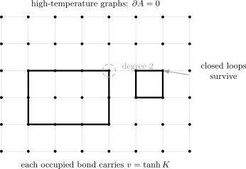
In the high-temperature expansion, every selected bond contributes a factor $v=\tanh K$. The spin sum kills any graph with an odd number of selected bonds incident on some site. The surviving graphs are closed even subgraphs, which are loop configurations on a square lattice.

The name “high-temperature expansion” comes from the fact that $v=\tanh K$ is small when $K=\beta J$ is small. The leading term is the empty graph,

$$Z(K)=2^{N_s}(\cosh K)^{N_b} \left(1+\text{small loops}+\cdots\right).$$

For a simply connected square lattice, the smallest local loop is a plaquette of length $4$, so the first local correction is of order $v^4$. On a small torus, winding loops are additional finite-size contributions.

The crucial point is that this expansion is not a perturbation expansion in a continuum coupling. It is an exact combinatorial identity, followed by a useful approximation when $v$ is small. The objects being counted are geometrical: closed loops on the lattice.

Spin correlators as open graphs

The same expansion gives a clean interpretation of spin correlation functions. Consider two spins at sites $x$ and $y$:

$$\langle \sigma_x\sigma_y\rangle ={1\over Z} \sum_{\{\sigma\}}\sigma_x\sigma_y \prod_{\langle ij\rangle} e^{K\sigma_i\sigma_j}.$$

Repeating the high-temperature expansion gives

$$\langle \sigma_x\sigma_y\rangle = { \sum_{A:\partial A=\{x,y\}} v^{|A|} \over \sum_{A:\partial A=0} v^{|A|} }.$$

The numerator is no longer a sum over closed graphs. Because of the extra insertion $\sigma_x\sigma_y$, the surviving graphs must have odd degree at $x$ and $y$, and even degree everywhere else. Thus $A$ contains an open path from $x$ to $y$, possibly decorated by closed loops.

This is the first appearance of a pattern that will recur repeatedly:

$$\text{partition function}\quad \leftrightarrow \quad \text{closed objects},$$

while

$$\text{correlator with insertions}\quad \leftrightarrow \quad \text{objects ending on the insertions}.$$

At high temperature, the leading contribution to $\langle \sigma_x\sigma_y\rangle$ comes from shortest paths connecting $x$ and $y$. If $r=|x-y|_1$ is the Manhattan distance on the square lattice, then

$$\langle \sigma_x\sigma_y\rangle \sim N_{\text{paths}}(x,y) (\tanh K)^r+\cdots,$$

where $N_{\text{paths}}(x,y)$ counts shortest lattice paths. Along a lattice axis this multiplicity is one, and at strictly leading order as $K\to0$,

$$(\tanh K)^r=e^{-r/\xi_{\text{HT}}}, \qquad \xi_{\text{axis}}^{-1}=-\log(\tanh K)+O\big((\tanh K)^2\big).$$

For other directions, the exponential growth of the number of paths modifies the numerical inverse correlation length. The robust conclusion is that sufficiently high temperature has a finite correlation length; the exact correlation length near criticality requires summing graphs of all sizes.

The exact correlation length near criticality is not given by this first term; near the transition, loops of all sizes contribute. But the leading high-temperature term correctly teaches the physical mechanism: correlations are carried by paths, and the path tension is set by $-\log\tanh K$.

Low-temperature expansion

The low-temperature expansion starts from the opposite limit. When $K$ is large, the dominant configurations are close to one of the two ordered ground states. Let us first impose $+$ boundary conditions, so the system is forced to be in the $+$ phase near the boundary. A configuration with some flipped spins contains islands of $-$ spins inside a sea of $+$ spins.

Every bond joining unlike spins is broken. If $L(\mathcal C)$ is the number of broken bonds, then

$$\sum_{\langle ij\rangle}\sigma_i\sigma_j =N_b-2L(\mathcal C).$$

Indeed, each satisfied bond contributes $+1$, while each broken bond contributes $-1$; replacing a satisfied bond by a broken one changes the sum by $-2$. Therefore

$$e^{K\sum_{\langle ij\rangle}\sigma_i\sigma_j} =e^{K N_b}e^{-2K L(\mathcal C)}.$$

On the square lattice, broken bonds are crossed by closed contours on the dual lattice. These contours are the domain walls separating $+$ and $-$ domains. With $+$ boundary conditions, the low-temperature expansion is

$$\boxed{ Z_+(K)=e^{K N_b} \sum_{\mathcal C} e^{-2K L(\mathcal C)}. }$$

Here $\mathcal C$ is the occupied dual-edge set separating opposite spins. It has even degree at every interior dual vertex; choosing how to pair four edges at an intersection is only a drawing convention. With periodic boundary conditions, every compatible wall set has a globally reversed partner, but the wall set must be trivial in $\mathbb Z_2$ homology. With free boundary conditions, interfaces may end on the boundary. Thus the displayed closed-contour formula is specifically the clean $+$-boundary version.

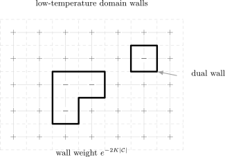
In the low-temperature expansion, the elementary excitation is a domain wall. Each broken bond costs energy $2J$, so a contour configuration $\mathcal C$ has Boltzmann weight $e^{-2K L(\mathcal C)}$, where $L(\mathcal C)$ is the total contour length.

The low-temperature expansion is again an exact geometrical rewriting, not merely a picture. Its small parameter is

$$e^{-2K}=e^{-2\beta J},$$

which is the Boltzmann weight for one broken bond. At very low temperature, long contours are suppressed.

For a single droplet, the energy cost is proportional to its boundary length, not its area:

$$\Delta H=2J L.$$

This distinction is important. Flipping a compact region of $A$ spins does not cost energy proportional to $A$; it costs energy proportional to the size of the interface. The system resists domain formation by surface tension.

Energy, entropy, and the Peierls intuition

If only energy mattered, the ordered phase at low temperature would be obvious: long domain walls cost $2K L$ in the exponent. But statistical mechanics is never only energy. There are many possible loops of a given length. If the number of loops of length $L$ grows like

$$N(L)\sim e^{sL},$$

then the total contribution of loops of length $L$ behaves roughly like

$$N(L)e^{-2KL}\sim e^{-(2K-s)L}.$$

The constant $s$ is an entropy per unit length. Large loops are suppressed if

$$2K>s.$$

They proliferate if the entropic gain overwhelms the energetic cost. This single-parameter estimate is heuristic: the entropy density depends on which contours are counted and on their interactions, so $2K=s$ is not an exact determination of $K_c$.

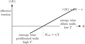
A domain wall of length $L$ has energy cost $2K L$ in the Boltzmann exponent, but the number of possible walls grows exponentially with $L$. In the dilute-wall estimate, the effective tension is $2K-s$; its zero is only a heuristic threshold, not the exact critical coupling.

This is the basic Peierls argument. Fix a local rule for resolving any degree-four meeting into non-self-intersecting contours, and impose $+$ boundary conditions. If the spin at the origin is $-$, then at least one resolved contour surrounds the origin. Hence

$$\mathbb P(\sigma_0=-1) \le \sum_{\gamma\text{ surrounds }0} e^{-2K|\gamma|}.$$

On the square lattice, the number of contours of length $L$ surrounding a fixed point can be bounded by $C L3^L$. The polynomial factor accounts for choosing a marked crossing or starting edge; after that choice, there are at most three non-backtracking continuations at each step. Therefore

$$\mathbb P(\sigma_0=-1) \le C\sum_{L\ge 4} L\,3^L e^{-2KL}.$$

For sufficiently large $K$, this series is small. Then

$$\langle \sigma_0\rangle_+ =1-2\mathbb P(\sigma_0=-1)>0.$$

This proves the existence of a low-temperature ordered phase in two dimensions. The proof is deliberately rough; it does not locate the exact critical point. Its virtue is conceptual: it shows why a finite-temperature phase transition is possible. Domain walls have a tension, and in $d\ge2$ the cost of a large droplet grows with its boundary.

Why one dimension has no transition

The one-dimensional Ising model is the best warning against overinterpreting finite domains. Consider an open chain of $N$ spins:

$$H=-J\sum_{i=1}^{N-1}\sigma_i\sigma_{i+1}.$$

A domain wall is now just a point: a bond across which the spin changes sign. If there are $n$ domain walls, then

$$H=-J(N-1)+2Jn.$$

The partition function is exactly

$$Z_N =2e^{K(N-1)} \sum_{n=0}^{N-1}{N-1\choose n}e^{-2Kn} =2e^{K(N-1)}(1+e^{-2K})^{N-1}.$$

Equivalently,

$$Z_N=2(2\cosh K)^{N-1}.$$

At any finite $K$, the density of domain walls is nonzero:

$$\rho_{\text{wall}} ={e^{-2K}\over 1+e^{-2K}}.$$

Even if $K$ is large, the chain has a typical domain size of order $e^{2K}$, which is large but finite. In an infinite chain, infinitely many domain walls appear at any nonzero temperature, so long-range order is destroyed.

The two-point function can be computed exactly:

$$\langle \sigma_0\sigma_r\rangle=(\tanh K)^r.$$

Thus the correlation length is

$$\xi^{-1}=-\log(\tanh K),$$

which is finite for every finite $K$. The only singular point is $K=\infty$, or zero temperature. This is why one-dimensional short-range Ising systems have no finite-temperature phase transition.

The contrast with two dimensions is sharp. In one dimension, a large reversed interval costs only the energy of two domain walls, independent of its length. In two dimensions, a large droplet costs energy proportional to its perimeter. The interface tension can defeat entropy at low temperature.

Higher dimensions and random surfaces

In $d$ dimensions, low-temperature domain walls are $(d-1)$-dimensional objects. In two dimensions they are loops. In three dimensions they are closed surfaces. On a cubic lattice, a flipped droplet is surrounded by plaquettes of the dual lattice, and the weight is

$$e^{-2K A},$$

where $A$ is the number of dual plaquettes in the interface.

This observation is one of the reasons the Ising model is such a natural starting point for this course. It connects ordinary phase transitions to sums over extended objects:

$$\begin{array}{ccl} \text{high-temperature expansion} & \longrightarrow& \text{closed lattice paths},\\ \text{two-dimensional low-temperature expansion} & \longrightarrow& \text{closed domain-wall loops},\\ \text{three-dimensional low-temperature expansion} & \longrightarrow& \text{random closed surfaces}. \end{array}$$

A random surface weighted by area is already string-like. Of course, an Ising domain wall is not yet a fundamental string. It lives on a lattice, may have short-distance self-intersections depending on the contour convention, and comes with microscopic weights inherited from the spin model. But the structural resemblance is important: a statistical system can generate a sum over fluctuating geometries.

Later in the course, Wilson loops, random lattices, compact gauge fields, and worldsheet path integrals will make this relation much more precise. The Ising model gives the first clean version: fields can be traded for geometry, and geometry can carry correlations.

From graphical expansions to criticality

The high- and low-temperature expansions are most useful when their geometrical objects are dilute. At high temperature, the loop fugacity $v=\tanh K$ is small. At low temperature, the domain-wall fugacity $e^{-2K}$ is small.

A phase transition occurs when neither picture is dilute. Loops or domain walls of arbitrarily large size become important. The correlation length diverges:

$$\xi\to\infty.$$

At that point, microscopic lattice details become less important than the long-distance scaling structure. This is the bridge to continuum field theory. In the Ising universality class, the long-distance effective action is organized by a scalar order-parameter field $\phi$ with $\mathbb Z_2$ symmetry,

$$\phi\mapsto-\phi,$$

and Euclidean action of the form

$$S_E[\phi]=\int d^d x\left[ {1\over2}(\partial\phi)^2+{1\over2}r\phi^2+{u\over4!}\phi^4+\cdots \right].$$

The field $\phi$ is not one microscopic spin. It is a coarse-grained magnetization. The parameter $r$ measures the distance from criticality, and the dots denote all additional local operators allowed by $\mathbb Z_2$ symmetry. The renormalization group will decide which of those terms matter at long distances.

This page stops before that continuum construction. The important point for now is that the Ising model already has two complementary nonperturbative descriptions:

$$Z \sim \sum_{\text{closed loops}}(\text{line fugacity})^{\text{length}} \sim \sum_{\text{domain walls}}e^{-\text{tension}\times\text{area or length}}.$$

These are the first examples of a principle that will keep returning: the right degrees of freedom depend on the regime.

Summary

The ferromagnetic Ising model has spins $\sigma_i=\pm1$ and global $\mathbb Z_2$ symmetry. Its partition function admits two exact graphical expansions.

At high temperature,

$$Z(K)=2^{N_s}(\cosh K)^{N_b} \sum_{A:\partial A=0}(\tanh K)^{|A|}.$$

The surviving graphs are closed even subgraphs because the spin sum vanishes unless each site is touched by an even number of occupied bonds. Spin correlators are represented by open graphs whose endpoints sit at the operator insertions.

At low temperature, with $+$ boundary conditions,

$$Z_+(K)=e^{K N_b} \sum_{\mathcal C} e^{-2K L(\mathcal C)}.$$

The configurations $\mathcal C$ are domain walls on the dual lattice. Each broken bond costs $2J$, so the Boltzmann weight is controlled by the total contour length. In three dimensions, these domain walls become random surfaces.

The possibility of a phase transition is an energy–entropy question. Domain walls cost energy proportional to their size, but the number of possible walls also grows exponentially. In one dimension, domain walls are point defects with finite density at any nonzero temperature, and there is no finite-temperature phase transition. In two and higher dimensions, interface tension can stabilize an ordered phase at low temperature.

Common pitfalls

Treating the high-temperature expansion as approximate. The graph identity is exact before truncation. The approximation enters only when one keeps a limited set of short graphs because $\tanh K$ is small.

Equating an even subgraph with a simple loop. A surviving edge set may have disconnected components, winding sectors, or degree-four vertices. Pairing edges into individual loops at an intersection is not unique, but the even subgraph itself is.

Counting flipped spins instead of broken bonds. The energy cost of a droplet is proportional to its interface, not its volume. Boundary conditions determine whether that interface must close or may end at the system boundary.

Assigning spontaneous magnetization to a finite system. At zero field a finite system retains the exact $\mathbb Z_2$ symmetry and has vanishing one-point function. The ordered phase requires the thermodynamic limit before the symmetry-breaking field is removed.

Reading the Peierls estimate as the exact transition. The entropy count is deliberately crude and proves order only for sufficiently large $K$. It does not determine the square-lattice value of $K_c$.

Importing one-dimensional intuition into higher dimensions. A domain wall in one dimension is pointlike and has finite density at every nonzero temperature. In two dimensions its energy grows with contour length, allowing interface tension to stabilize order.

Exercises

Exercise 1

Let $G=(V,E)$ be an arbitrary finite graph and define the Ising partition function

$$Z_G(K)=\sum_{\{\sigma\}}\prod_{\langle ij\rangle\in E} e^{K\sigma_i\sigma_j}.$$

Show that

$$Z_G(K)=2^{|V|}(\cosh K)^{|E|} \sum_{A:\partial A=0}(\tanh K)^{|A|},$$

where $\partial A$ is the set of vertices incident on an odd number of occupied edges in $A$.

Solution

Use

$$e^{K\sigma_i\sigma_j}=\cosh K(1+v\sigma_i\sigma_j), \qquad v=\tanh K.$$

Then

$$Z_G(K)=(\cosh K)^{|E|} \sum_{\{\sigma\}} \sum_{A\subset E}v^{|A|} \prod_{\langle ij\rangle\in A}\sigma_i\sigma_j.$$

Regrouping the spin factors gives

$$\prod_{\langle ij\rangle\in A}\sigma_i\sigma_j =\prod_{i\in V}\sigma_i^{d_A(i)},$$

where $d_A(i)$ is the number of occupied edges incident on $i$. The spin sums factorize:

$$\sum_{\{\sigma\}}\prod_i \sigma_i^{d_A(i)} =\prod_i\sum_{\sigma_i=\pm1}\sigma_i^{d_A(i)}.$$

Each factor is $2$ if $d_A(i)$ is even and $0$ otherwise. Thus only subsets with $\partial A=0$ survive, and each surviving subset contributes $2^{|V|}v^{|A|}$. This proves the formula.

Exercise 2

Using the high-temperature expansion, show that for two spin insertions on a finite graph,

$$\langle \sigma_x\sigma_y\rangle = { \sum_{A:\partial A=\{x,y\}} v^{|A|} \over \sum_{A:\partial A=0} v^{|A|} }, \qquad v=\tanh K.$$

Then explain why, at very high temperature on a square lattice, the leading contribution decays as $(\tanh K)^r$, where $r$ is the lattice distance between $x$ and $y$.

Solution

The numerator is

$$\sum_{\{\sigma\}}\sigma_x\sigma_y \prod_{\langle ij\rangle}e^{K\sigma_i\sigma_j}.$$

After expanding the bond factors, the spin power at a vertex $i$ is $d_A(i)$, except at $x$ and $y$, where the extra insertions add one additional power of $\sigma$. Therefore the spin sum is nonzero exactly when

$$d_A(i)\equiv0\pmod 2\quad (i\neq x,y), \qquad d_A(x)\equiv d_A(y)\equiv1\pmod 2.$$

Equivalently, $\partial A=\{x,y\}$. The common prefactor $2^{N_s}(\cosh K)^{N_b}$ cancels against the same prefactor in $Z$, giving the stated ratio.

For small $v$, the dominant numerator graphs have the fewest occupied bonds. Such a graph must contain a path from $x$ to $y$, so its length is at least the lattice distance $r$. The leading terms are shortest paths and contribute proportional to $v^r=(\tanh K)^r$. Longer paths and closed-loop decorations are higher order in $v$.

Exercise 3

Consider the square-lattice Ising model with $+$ boundary conditions. Suppose a configuration contains one droplet of $-$ spins whose Peierls contour has length $L$. Show that the energy cost relative to the all-$+$ configuration is $2JL$. Then use the rough bound $N(L)\le CL3^L$ for the number of contours of length $L$ surrounding the origin to explain why $\langle \sigma_0\rangle_+>0$ at sufficiently low temperature.

Solution

In the all-$+$ configuration, every bond is satisfied and contributes $-J$ to the Hamiltonian. A bond across the boundary of the droplet has opposite spins and contributes $+J$. Replacing one satisfied bond by one broken bond raises the energy by

$$(+J)-(-J)=2J.$$

If the contour crosses $L$ broken bonds, then

$$\Delta H=2JL.$$

The Boltzmann suppression is therefore $e^{-2KL}$. If $\sigma_0=-1$, then the origin must be enclosed by at least one contour. Hence

$$\mathbb P(\sigma_0=-1) \le \sum_{L\ge4} N(L)e^{-2KL} \le C\sum_{L\ge4}L\,3^L e^{-2KL}.$$

The geometric series converges when $3e^{-2K}<1$, and it becomes small for large $K$. Therefore

$$\langle \sigma_0\rangle_+ =1-2\mathbb P(\sigma_0=-1)$$

is positive at sufficiently low temperature. This is the Peierls mechanism for spontaneous magnetization.

Exercise 4

For the one-dimensional Ising chain with open boundary conditions,

$$H=-J\sum_{i=1}^{N-1}\sigma_i\sigma_{i+1},$$

derive

$$Z_N=2e^{K(N-1)}(1+e^{-2K})^{N-1} =2(2\cosh K)^{N-1}.$$

Then show that the domain-wall density is finite for every finite $K$.

Solution

A domain wall occurs on a bond where $\sigma_i\neq \sigma_{i+1}$. If there are $n$ domain walls, then $n$ bonds are broken and $N-1-n$ bonds are satisfied. The energy is

$$H=-J(N-1-n)+Jn=-J(N-1)+2Jn.$$

Choose the positions of the $n$ walls in ${N-1\choose n}$ ways. Once the first spin is chosen, the wall positions determine all remaining spins, giving an overall factor $2$. Therefore

$$Z_N=2\sum_{n=0}^{N-1}{N-1\choose n} e^{K(N-1)}e^{-2Kn} =2e^{K(N-1)}(1+e^{-2K})^{N-1}.$$

Since

$$e^K(1+e^{-2K})=e^K+e^{-K}=2\cosh K,$$

this is also $2(2\cosh K)^{N-1}$.

The mean wall density is obtained from the binomial distribution with wall fugacity $q=e^{-2K}$:

$$\rho_{\text{wall}}={q\over1+q}={e^{-2K}\over1+e^{-2K}}.$$

This is nonzero for every finite $K$. Hence an infinite chain contains a finite density of domain walls at any nonzero temperature, and long-range order is absent.

References

• Robert B. Griffiths, “Peierls Proof of Spontaneous Magnetization in a Two-Dimensional Ising Ferromagnet,” Physical Review 136 (1964), A437–A439.
• Rudolf Peierls, “On Ising’s Model of Ferromagnetism,” Mathematical Proceedings of the Cambridge Philosophical Society 32 (1936), 477–481.

Further reading

• Leo P. Kadanoff, “Scaling Laws for Ising Models near $T_c$,” Physics 2 (1966), 263–272.
• Barry M. McCoy and Tai Tsun Wu, The Two-Dimensional Ising Model, Harvard University Press, 1973.
• Alexander M. Polyakov, Gauge Fields and Strings, Harwood Academic Publishers, 1987, Chapters 1, 3, and 10.
• Kenneth G. Wilson and John Kogut, “The Renormalization Group and the $\epsilon$ Expansion,” Physics Reports 12 (1974), 75–199.
• Jean Zinn-Justin, Quantum Field Theory and Critical Phenomena, 5th ed., Oxford University Press, 2021, Chapters 14–16.

References

Section titled “References”- Robert B. Griffiths, “Peierls Proof of Spontaneous Magnetization in a Two-Dimensional Ising Ferromagnet,” Physical Review 136 (1964), A437–A439. doi:10.1103/PhysRev.136.A437. Open PDF.