

Gauge-Invariant Observables and Asymptotic Amplitudes
Gauge-dependent fields are useful for calculations, but an observable must be defined independently of the redundant description. In this lesson, an Abelian Wilson line completes a neutral charged-field bilocal, an isolated particle pole permits scalar LSZ reduction, and intrinsic distance supplies a relational question in a regulated Euclidean geometry integral. The distance-weighted pair observable is not automatically a normalized average, and its Laplace kernel is not an exact massive propagator.
The worldline construction supplies the normalized Euclidean heat kernel used below. The source-response convention fixes and its contact terms. For the distinction between redundant gauge transformations and physical boundary charges, see Gauge-invariant dressed observables.
Gauge-invariant content in QED
Section titled “Gauge-invariant content in QED”Orient the Abelian Wilson line from to :
This is endpoint covariance at operator level. An open line alone is not gauge-invariant. Its completed neutral bilocal is:
because the factors from and cancel the two endpoint phases. Exercise 1 gives the cancellation explicitly. A transformation law for a gauge-fixed expectation value would additionally require specifying how its gauge-fixing and background data change.
The bilocal has zero total charge and depends on the chosen path. Two finite paths with the same endpoints differ by a closed Wilson holonomy; that difference need not change fields arbitrarily far away. By contrast, an operator creating a single charged excitation needs a nonlocal dressing to a boundary or an appropriate Coulomb field. Gauss’s law prevents a compactly supported local observable from creating a nonzero asymptotic electric charge.
Here gauge invariance means invariance under the redundancy subgroup , with the prescribed boundary behavior. A transformation with a nonzero physical boundary charge is not automatically in . A charged dressing can be invariant under and still transform under that boundary symmetry. Formal endpoint cancellation does not by itself construct a finite-energy charged state or its infrared scattering prescription.
In Abelian theory, local neutral operators such as and , closed Wilson loops, and endpoint-completed lines are useful invariant quantities. Non-Abelian field-strength components are instead gauge-covariant and need invariant contractions or traces. These distinctions matter before interpreting a gauge-fixed propagator as physical data.
On-shell amplitudes from gauge-dependent fields
Section titled “On-shell amplitudes from gauge-dependent fields”For a Hermitian scalar in a positive-metric Lorentzian vacuum theory, assume a stable isolated one-particle state, a nonzero interpolating-field overlap, and well-defined in/out wave packets whose residual interactions become negligible at asymptotic times. These are scattering assumptions, not ultraviolet asymptotic freedom; In and out states explains their limits. Use and choose the particle-state phase so that
The two-point residue has two overlaps, one at each end. Each external leg of a connected -point function instead has the factor . With incoming and outgoing Fourier phases chosen consistently, its simultaneous external-pole part is
Thus multiply by for every leg and take the pole limit. The result is times the momentum-conserving delta function. The subscript selects connected scattering; subtracting the identity from the full S-matrix alone does not remove every disconnected scattering cluster.
The normalization can be checked directly. Apply the unit-overlap LSZ formula to . For each leg, integration by parts gives
The incoming phase is negative and the outgoing phase positive. This projects the time-ordered function onto its asymptotic particle poles. Schwartz 2014, §6.1, pp.70–74 derives the reduction and explains interpolating operators; his generalized-operator discussion calls the overlap itself . Here denotes its squared magnitude, the pole residue. The explicit factors therefore follow from the normalization just given. The scalar LSZ account develops the full packet and connected-state construction in the same convention.
In gauge theories, residues of gauge-variant fields can depend on gauge fixing. Physical poles and complete amplitudes between admissible physical states must be independent of it, with fixed physical inputs and the appropriate anomaly-free Ward or BRST identities. This is a condition on the complete calculation, not on each off-shell factor; the relevant qualifications are developed in BRST cohomology and physical observables.
For example, the QED polarization tensor is transverse,
The explicit one-loop transverse structure appears in Schwartz 2014, p.309, Eq.16.47. In a Euclidean cutoff calculation, an uncancelled local term proportional to would violate this identity. A cutoff that breaks momentum-shift identities can generate such terms. Symmetry-restoring counterterms require the actual locality and anomaly conditions; a nontransverse result is not acceptable merely because its integrals are finite. Exercise 5 isolates this diagnostic.
Massless QED also limits the particle-pole picture. Its charged sector has infraparticle behavior, and scattering between naive charged Fock states is infrared ill-defined. Inclusive probabilities or appropriately dressed asymptotic states address different physical questions. The scalar isolated-pole formula above is not a derivation of either construction.
Gravity: coordinates are also gauge data
Section titled “Gravity: coordinates are also gauge data”In a dynamical geometry, transformations in the diffeomorphism redundancy group move the metric and matter together while preserving the specified boundary data. Scalar covariance says
This relates two descriptions of the same value; it does not identify a physical insertion by the bare coordinate label . In particular, a curvature scalar is not made into an invariant local insertion merely by being a scalar. The point must be identified by boundary anchoring, matter clocks and rods, geometric relations, or an invariant integration prescription.
A gauge-fixed graviton correlator is likewise a useful intermediate object. At linear order, the redundancy includes
Changing this description is distinct from acting with a physical asymptotic symmetry. The relational and boundary observable discussion explains that distinction beyond the elementary example here.
Asymptotic observables
Section titled “Asymptotic observables”The available asymptotic data depend on the spacetime and boundary conditions:
- In asymptotically flat spacetime, an S-matrix is a natural candidate when appropriate in/out states exist. Massless gauge fields and gravity require an infrared prescription; boundary charges and soft data are not simply discarded as gauge redundancy.
- Anti-de Sitter space has a timelike conformal boundary. With specified boundary conditions and renormalized sources, boundary responses and correlators are natural data. They are not a generic flat-space S-matrix.
- In de Sitter settings, one often studies wavefunction coefficients, late-time correlators or in-in expectation values rather than the same flat-space in/out S-matrix. Their state, gauge and boundary prescriptions remain part of the question.
These are possible formulations of observables, not interchangeable answers to every gravitational scattering problem.
Relational correlators in fluctuating geometry
Section titled “Relational correlators in fluctuating geometry”The geometric step can be seen before averaging over any metrics. Consider one flat Euclidean plane with dimensionless coordinates and positive length scale :
The inverse is , , and the Jacobian determinant is one. In the new coordinates,
The same path from to has descriptions and , for . Its transformed tangent is , so
The inverse map takes every competing path back to one between the same endpoints in the flat plane, where the straight segment minimizes length. Thus the mapped path remains a minimizing geodesic. Inspect how the figure transforms the whole reference grid and the path together; their bent coordinate images do not imply physical curvature.
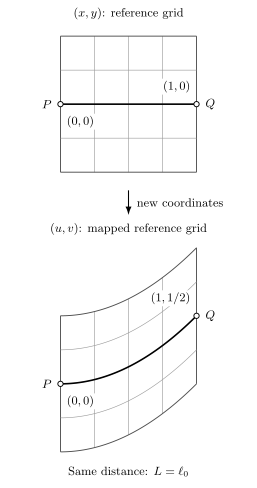
One flat geometry in two coordinate charts. The highlighted path joins the same physical points and ; the lower panel maps every reference-grid line and the path by , . With the transformed metric, the distance is in both charts. Lengths measured with the lower drawing’s Euclidean paper metric are not physical lengths. This is a kinematical coordinate example, not an average over geometries.
Now let denote insertion points in a -dimensional Euclidean metric ensemble. Assume positive nondegenerate metrics, a regulated measure and action invariant under the anomaly-free redundancy group , and either a closed finite-volume geometry or specified boundary and infrared conditions. The quotient below is formal notation for a compatible gauge-fixing prescription, not a proof that the quantum-gravity integral exists. Let be renormalized scalar operators, not scalar densities, and take :
Here is the same regulated integral without insertions; whenever an ordinary expectation value is used, assume this normalization is finite and nonzero. The invariant measures, scalar insertions and intrinsic distance make this a distance-weighted pair observable. It still needs the appropriate composite/contact renormalization; cut loci or boundary prescriptions can matter. Its distance is physical metric data, so this construction is not invariant under an additional independent Weyl gauge transformation.
The expression is a pair density, not a normalized conditional mean. When is finite and nonzero, one may instead form
This is a pair-normalized average. If and denote the operator units, then and . A conditional probabilistic interpretation additionally requires a positive normalized ensemble, which the formal gravitational integral has not established.
There is a useful exact check on a fixed flat torus of volume . For and below the torus’s injectivity radius, the sphere of radius around each point is an ordinary Euclidean sphere. Consequently,
where is the area of the unit -sphere. The unnormalized observable counts the available shell of pairs; the ratio removes that geometric density.
Distance weights and massive probes
Section titled “Distance weights and massive probes”For a positive inverse-length parameter , whenever the transform converges and the integrations can be interchanged,
This identity is exact. Its exponential kernel is not the full massive scalar propagator. To see the difference, take a free scalar on , , and . The normalized proper-time representation is
Here has units length squared; the separation above has units length. In the worldline lesson’s notation, is half the einbein modulus, not half a geodesic distance. The normalized kernel and this conversion are derived in the worldline lesson; the regulated random-path construction reaches the inverse scalar denominator in Polyakov 1987, §9.2, p.163, Eq.9.46.
The exponent has the saddle
It explains the leading exponential at large , but the kernel and fluctuations also supply a prefactor. In three flat dimensions the exact answer is
For , substitution into verifies the radial equation. The outward flux of through a shrinking sphere tends to one, fixing the delta-function normalization at the origin. Thus even this simplest exact propagator differs from the raw Laplace weight by .
A heavy-probe interpretation on a smooth curved background is an approximation with further conditions: specified Green-function boundary data, a unique nonconjugate minimizing geodesic, large , and a short-proper-time saddle relative to curvature scales. Geometric prefactors, multiple geodesics and boundary contributions cannot generally be omitted. A fixed-background approximation also does not automatically hold uniformly inside an integral over metrics. The distance Laplace transform and a correlator constructed with an actual massive Green function are therefore distinct observables.
Sources, deformations, and effective actions
Section titled “Sources, deformations, and effective actions”For a real linear action source on a fixed background, define
For source-independent operators, differentiation gives
Source dependence of the action, operators or local counterterms adds the corresponding contact terms. The second connected derivative has a minus sign for the declared convention.
In gravity, the measure and source must also be specified covariantly. A source can transform as external data; holding a bare coordinate-dependent function fixed does not define a diffeomorphism-invariant deformation by itself. Constant couplings to integrated scalars give formal invariant deformations of the regulated ensemble:
Their renormalization and the existence of the integral remain separate from this covariance argument. Likewise, a coordinate-momentum cutoff is not made covariant merely by shifting its argument by a local gauge potential. The action, measure and counterterms must satisfy the relevant Ward identities.
Why random lattices enter
Section titled “Why random lattices enter”A finite lattice can turn a field integral into finitely many integrations, but convergence still depends on the action, zero modes and volume prescription. A fixed metric square lattice does not itself sum over geometry. This does not exclude discretizations with fixed combinatorics and fluctuating lengths.
The route taken next is a sum over two-dimensional discretized surfaces. Ribbon graphs carry a cyclic ordering at their vertices; their thickening supplies faces and topology. With specified edge/face data and weights, they can represent an ensemble of geometries. An arbitrary irregular graph does not provide all of these structures, and summing graphs does not by itself prove restoration of a desired continuum symmetry. The next lesson develops the matrix-model construction.
Exercises
Section titled “Exercises”Exercise 1: Wilson-line cancellation of endpoint phases
Section titled “Exercise 1: Wilson-line cancellation of endpoint phases”Using the global Abelian convention and the oriented path from to , show that
is gauge-invariant.
Solution
Under
the Wilson line transforms as
Therefore
and all phases cancel. Thus is gauge-invariant.
Exercise 2: Amputation and external-state normalization in LSZ
Section titled “Exercise 2: Amputation and external-state normalization in LSZ”Assume a normalized physical scalar state with an isolated stable pole, nonzero , and an admissible asymptotic-state construction as above. Suppose the exact two-point function has the pole
Explain why the factor appears for each external scalar leg in LSZ reduction.
Solution
In a two-point function the isolated pole has residue because there is an overlap at each end. In a general time-ordered -point function, the factor associated with one external leg is instead schematically
times the matrix element for the remaining process. The pole reflects propagation of an asymptotic one-particle state created by the field. Multiplying by removes the propagator denominator, and multiplying by removes the overlap of the interpolating field with the normalized external state, up to the standard phases and factors of .
The field does not create a normalized one-particle state with unit amplitude; it creates it with overlap :
Therefore the combination is precisely the operation of amputating the pole and normalizing the external state. This derivation assumes an isolated stable-particle pole; the charged infraparticle sector of massless QED requires a dressed or inclusive treatment instead.
Exercise 3: Why a scalar at a coordinate point is not observable
Section titled “Exercise 3: Why a scalar at a coordinate point is not observable”Let be a scalar field in a dynamical geometry, and restrict the diffeomorphisms in this question to the redundancy subgroup preserving the specified boundary data. Why is at an unanchored coordinate label not by itself an invariant observable, even though is a scalar?
Solution
A scalar field has the transformation law
under a diffeomorphism . This means the value of the field at the physical point is invariant, but the coordinate label of that point changes.
The expression with fixed coordinate label assumes that has physical meaning. In a theory of dynamical geometry, diffeomorphisms are gauge redundancies, so two configurations related by moving the coordinate label represent the same physical configuration. Therefore a local insertion at a bare coordinate point is gauge-dependent.
To make an observable, one must identify the point relationally, anchor it to boundary data, or integrate over positions with an invariant measure.
Exercise 4: Diffeomorphism invariance of a geodesic-distance correlator
Section titled “Exercise 4: Diffeomorphism invariance of a geodesic-distance correlator”For the regulated Euclidean ensemble above, show that the distance-weighted pair observable
is invariant under redundancy diffeomorphisms, assuming and are scalar operators and the regulated measure, action, integration domain and composite prescription respect those transformations. Use the stated closed-manifold or fixed-boundary conditions. The two factors mean and , respectively.
Solution
Under a diffeomorphism, the volume element is invariant as a density:
Scalar operators satisfy
The geodesic distance is an intrinsic quantity, so
Therefore every factor in the integrand transforms covariantly, and after changing integration variables from to , the value of the integral is unchanged. The delta function imposes a condition on an invariant distance, not on coordinate separation.
Exercise 5: Detecting a gauge-violating photon mass term
Section titled “Exercise 5: Detecting a gauge-violating photon mass term”In ordinary unbroken, anomaly-free QED, suppose a Euclidean cutoff calculation leaves the following local mass term in the polarization tensor. A dimensionless loop coefficient is suppressed; indices in this exercise are Euclidean:
Why is the first term incompatible with gauge invariance?
Solution
Gauge invariance implies the Ward identity
The transverse structure satisfies this identity:
The cutoff term gives
which is nonzero. It is equivalent to generating a photon mass term
which is forbidden by gauge invariance. A gauge-invariant regulator avoids such a term, or the term must be subtracted by enforcing the Ward identity.