

Leading Logarithms and Nested Subgraphs
The previous page found the first ultraviolet logarithm in four-dimensional theory. We study the marginal four-point coupling in an infrared-safe Euclidean regime with a common scale , fixed dimensionless kinematic ratios, and positive weak coupling throughout the flow. A one-loop bubble gives
so the four-point vertex contains a correction of order . A single logarithm is already enough to warn us that perturbation theory is not organized only by powers of . If the ratio of scales is very large, then
may be order one even when .
Higher ultraviolet logarithms arise from compatible scale hierarchies, described by forests of nested or disjoint divergent subgraphs. We work through a nested chain: a hard subgraph shrinks to a local vertex, a softer subgraph uses that vertex, and the process repeats. The ordered integrals explain the logarithmic powers; graph and channel sums determine their coefficients.
Required background. Scalar Propagators and One-Loop φ⁴ supplies the bubble symmetry factor, the three crossing channels, and the effective-action sign convention for the four-point vertex.
What counts as a leading logarithm
Section titled “What counts as a leading logarithm”Logarithmic variables and one-loop coefficient
Section titled “Logarithmic variables and one-loop coefficient”A positive mass or a suitable nonexceptional critical prescription must control the infrared regions. For a massive theory the massless running formula applies above the mass scale, not through the threshold to physical momentum zero. Keep all other scale ratios fixed; arbitrary soft, collinear, or multiscale logarithms are outside this ultraviolet classification. The distinction between single-scale RG logarithms and more general logarithms is discussed in Collins 1984/2023, §§ 7.6.1–7.6.2, pp. 193–196. We write
For real scalar theory in four Euclidean dimensions, the one-loop logarithmic correction to the four-point coupling is written as
The coefficient includes the three channels and the bubble symmetry factor . As on the previous page, is the Euclidean effective-action coefficient, with the bare coupling fixed at ; it is not the invariant scattering amplitude.
In this single-scale ultraviolet expansion, the -loop contribution has the schematic form
The leading-logarithmic approximation keeps only the highest power at each order:
It is designed for the scaling regime
In this regime,
so infinitely many loop orders can contribute at the same parametric size. Terms such as are smaller by one explicit power of and belong to next-to-leading-log accuracy.
This is why constants inside logarithms are unimportant at leading-log order. For example,
The first term may be large; the second is an ordinary finite number. At one loop the difference between and is only , while the leading-log term is treated as when .
Leading-log accuracy retains the enhanced terms while the running coupling remains weak. Finite matching constants enter at lower logarithmic accuracy; this organization does not assert convergence of the full perturbative series.
Ordered logarithmic integrals
Section titled “Ordered logarithmic integrals”The simplest source of a logarithm is the scale-invariant integral
If two independent variables each ranged freely from to , the integral would give . But loop momenta in a leading region are often not merely independent; they are ordered. For two ordered scales,
we find
The factor is the area of a triangle in logarithmic variables. Set
Then means , and the ordered region is half of the square . The figure’s full triangle represents strong ordering only to leading-log accuracy: it also includes comparable momenta near the diagonal. Removing a strip of fixed logarithmic width changes the area by , leaving the leading unchanged.
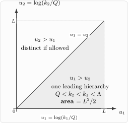
Two logarithmic integrations become an area in the plane of logarithmic momenta. The strongly ordered region occupies a triangle of area , where .
The triangle is one leading region, not the whole two-loop integration domain. If the graph also permits the opposite hierarchy , that is a second region; if the loop labels are related by a graph symmetry, its multiplicity must be included only once. Channel sums and insertion sites supply further combinatorial factors. The simplex volume therefore does not by itself determine the coefficient of a Feynman graph. It determines the logarithmic volume of one specified ordering.
For strongly ordered scales,
one obtains the volume of an -simplex:
This factorial is not an accident. It is the same combinatorial structure that appears when a differential RG equation is integrated repeatedly. The RG equation will be the efficient way of summing these ordered regions.
Toy integrals and the loss of constants
Section titled “Toy integrals and the loss of constants”The following toy integrals illustrate the loss of finite constants. Here and are dimensionless ratios to the fixed reference scale represented by . Consider
For large ,
At leading-log accuracy this is simply . The additive constant is finite and cannot be distinguished from other finite short-distance details.
Now consider the ordered two-variable version
Since the inner integral is , we have
The lesson is not tied to this particular integral. Whenever a loop region reduces to a scale-invariant measure , an ordered chain of such regions produces powers of logarithms. Leading logs remember only the large logarithmic volume; finite endpoints and smooth details are subleading.
Momentum shells in four dimensions
Section titled “Momentum shells in four dimensions”In four Euclidean dimensions,
after angular integration. Thus a one-loop logarithmic subgraph behaves like a shell integral:
For the one-loop four-point vertex in real theory, there are three channels and a symmetry factor , so the logarithmic shell coefficient becomes
when we use . This coefficient is the elementary building block for the leading logarithms of the four-point coupling.
At two loops and beyond, a large logarithm appears when at least one loop momentum can move through a wide range of scales while the rest of the integrand is approximately scale invariant. A double logarithm appears when two such scale variables can range over a two-dimensional logarithmic region. The crucial distinction is whether this two-dimensional region is broad in both directions or squeezed into a diagonal band.
Nested bubbles in φ⁴ theory
Section titled “Nested bubbles in φ⁴ theory”The most transparent two-loop leading-log region in theory is a bubble correction inserted into another bubble. Let be the hard loop momentum inside a subgraph and the softer loop momentum of the graph that contains it. The leading region is
The hard subgraph cannot resolve the external momenta of the softer graph. To the softer loop, it looks like a local correction to the four-point vertex. Thus the two-loop integral factorizes into two one-loop logarithmic integrations:
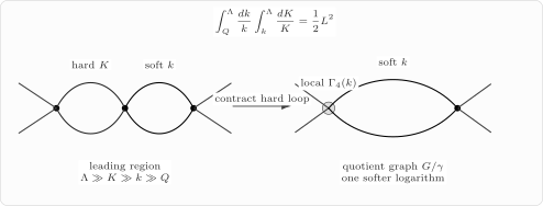
In the region , the hard loop with momentum shrinks to a local four-point vertex for the softer loop with momentum . This staged collapse is the diagrammatic origin of leading-log factorization.
To connect this with the coefficient , write the one-loop result schematically as
If a loop at scale uses a vertex already corrected by harder momenta , then to leading-log accuracy the effective vertex entering that softer loop is
The one-loop shell correction from the softer scale is proportional to in the natural logarithmic measure. Keeping terms through order gives
Integrating from to gives
Since
we get
The two-loop leading logarithm is therefore determined by the one-loop logarithm. This is the first visible hint that the entire leading-log series is not new information at every order.
Locality at each stage
Section titled “Locality at each stage”The factorization above relies on locality. Expand the hard integration region in its smaller external momenta: its leading term must have the form of an allowed local operator. This is a hard-region expansion, not a prescription to set all external momenta to zero in an unregulated massless integral. The local replacement lets a softer loop treat the hard subgraph as a corrected vertex.
When , the hard bubble has characteristic size , while the softer graph varies over distances of order . Since
the hard subgraph is effectively pointlike from the viewpoint of the softer graph.
In momentum space this means that the hard subgraph can be Taylor-expanded in the small external momenta flowing through it:
For leading logarithms of a marginal operator, only the local leading term matters. Terms with extra powers of correspond to higher-derivative operators and do not contribute to the same leading logarithm of the original marginal coupling.
This is why the nested graph reduces to an iteration of the one-loop four-point correction: the hard bubble produces the same local operator , and the softer loop then treats it as an ordinary vertex.
Subgraphs, quotient graphs, and forests
Section titled “Subgraphs, quotient graphs, and forests”A subgraph is a collection of vertices and internal lines of a Feynman graph. A subgraph is important for renormalization when it is superficially divergent and has the external-leg structure of an operator allowed in the effective action. In theory in four dimensions, the central example is the logarithmically divergent four-point subgraph.
If is much harder than the rest of the graph, it can be collapsed to a point. The resulting graph is called the quotient graph and is denoted . Symbolically,
A collection of divergent subgraphs that are mutually disjoint or nested is called a forest. Compatible forests organize the local subtractions; overlapping subgraphs belong to different terms, as in Collins 1984/2023, § 5.5.1, pp. 109–110. For example, a chain of logarithmic subgraphs
corresponds to ordered scales
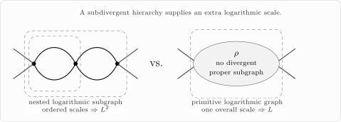
In the stated infrared-safe, single-scale ultraviolet regime, a nested logarithmic subgraph can supply a second ordered scale and generate . A primitive logarithmic graph with a finite ratio integral has one overall ultraviolet logarithm. The schematic comparison counts available scales, not the coefficient after graph sums.
Each hard subgraph in a forest is replaced by a local operator before the next softer integration. Corrections to that hard-region expansion carry powers of the small momentum ratios. The remaining softer graph still contains nonlocal momentum dependence; locality of the subtraction does not remove it.
Subtracting a nested subdivergence
Section titled “Subtracting a nested subdivergence”Let contain a proper logarithmically divergent four-point subgraph . The operator extracts its momentum-independent local subtraction coefficient, with the external-leg structure of . Use a hard-shell or infrared-safe subtraction prescription: zero-momentum Taylor subtraction in a massless graph can introduce infrared divergences (Collins 1984/2023, § 5.10, p. 135). Define its counterterm recursively by
Here means that any subdivergences inside have already been removed. For a graph with one proper nested subdivergence, the incomplete subtraction is
where is the quotient graph obtained by contracting to a local vertex. Only after this inner subtraction do we remove the overall local divergence:
The order matters: remove proper subdivergences before extracting the overall local counterterm. For a longer chain, proceed from the innermost subgraph outward. This recursive prescription is developed in Collins 1984/2023, § 5.3, pp. 101–104; the locality and finiteness discussion states the broader hypotheses.
There are two equivalent ways to use this structure at leading-log accuracy. In a renormalized graph, the local counterterm cancels the cutoff-dependent part of the hard subgraph, leaving a logarithm of physical or subtraction scales. In a Wilsonian calculation, the hard shell is integrated out and its local contribution is absorbed into the running vertex . The shell equation on the next page uses the second language. In both descriptions, the hard contribution is inserted once in ; this is what prevents double counting of the nested region.
Why primitive graphs give fewer logs
Section titled “Why primitive graphs give fewer logs”A primitive graph has no divergent proper subgraph. In the infrared-safe ultraviolet problem considered here, a primitive logarithmically divergent graph with a finite ratio integral has only one overall ultraviolet logarithm. For a multiloop graph this is below the highest possible logarithmic power; a one-loop primitive graph does give the leading one-loop logarithm.
The reason is simple in logarithmic variables. Suppose a two-loop primitive graph is logarithmically divergent overall. Introduce an overall scale and dimensionless ratios :
The logarithmic divergence comes from
If the ratio integral over is finite, there is only one overall ultraviolet logarithm. A compatible logarithmically divergent subgraph can provide another scale, for example in a hard hierarchy . A singular ratio endpoint caused instead by an uncontrolled infrared region lies outside this argument. The ultraviolet mechanism is:
The additional scale is a possible contribution; graph and channel coefficients may cancel. A toy model isolates the scale-counting distinction. Let
The kernel is broad neither in nor in independently; it is concentrated near the diagonal . For large ,
not . By contrast, the ordered region has area . These are log-volume models: the first has one wide overall scale, while the second permits a wide hierarchy.
Within this ultraviolet domain, multiloop graphs whose momenta remain comparable and which have no compatible logarithmic subhierarchies give lower powers of . The number of loops alone does not determine the logarithmic power.
This is one of the most useful calculation rules: leading logs are usually easier than full loop integrals because they ask only for scale-separated local limits. The full graph knows about constants, thresholds, tensor numerators, and regulator details; the leading log asks for the part that survives when each hard subgraph is shrunk to a point.
Overlapping subgraphs and leading logs
Section titled “Overlapping subgraphs and leading logs”Not all divergent subgraphs are neatly nested. Some overlap: they share internal lines but neither contains the other. Overlapping divergences are important for full renormalization, but they are not the basic source of a simple ordered leading-log chain.
In the stated ultraviolet regime, different hierarchies select different hard local subgraphs. Compatible forests organize the required subtractions without treating overlapping subgraphs as simultaneously nested. The nested chain explains the local recursion; it does not exhaust the forest formula or prove which coefficients survive the graph sum.
For the present course, the essential point is less formal:
Once a hard subgraph has been replaced by its local counterterm or local effective vertex, the remaining softer graph has the same form as a lower-loop problem. This recursive structure is why the renormalization-group equation will be first order in the scale.
Analytic continuation and cuts
Section titled “Analytic continuation and cuts”Analytic continuation gives a separate check on a specified logarithmic term. The following function is a zero-threshold log model, not a complete scattering amplitude. Euclidean calculations contain terms such as
For a Minkowski invariant , the model continues to
Fix a positive mass-squared reference . In the standalone logarithms below, denotes , denotes , and denotes . For on the principal branch,
so
With the discontinuity convention
the logarithm obeys
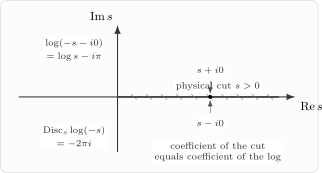
The illustrated logarithmic model has a cut starting at ; the image’s “physical cut” label refers to that model. It does not give the threshold of a massive two-particle channel. Boundary values are taken above and below the cut with the stated convention.
A physical channel containing two particles of equal mass instead has threshold (Srednicki 2006 draft, § 15, pp. 120–121, Eq. (15.5), PDF). Separately, let be a physical forward amplitude, with , normalized asymptotic states, and infrared-safe kinematics. With and phase space including the appropriate identical-particle factors, unitarity gives schematically
The specialization is essential for the left side to be twice an imaginary part; the general amplitude identity relates a matrix element to its adjoint. This physical statement does not assert that the massless forward limit is infrared safe, or identify with the Euclidean .
For a specified logarithmic term in such an amplitude, its discontinuity can fix its coefficient. Reconstructing the amplitude still requires local subtraction and matching data: cuts alone determine neither finite local constants nor an arbitrary full beta function. See the scope of cutting rules.
Example: the first three terms of the leading-log series
Section titled “Example: the first three terms of the leading-log series”Let
The one-loop result is
The leading two-loop term is generated by inserting the one-loop corrected vertex into the one-loop shell calculation, giving
Repeating once more gives
Thus the first leading-log terms organize as
which is the expansion of
at leading-log accuracy. The displayed series is its formal expansion; as a numerical geometric series it converges only for . The closed leading-log flow can be used beyond that series domain while the running coupling stays weak. The next lesson derives the scale equation and its kinematic domain.
Summary
Section titled “Summary”For the marginal four-point coupling in the infrared-safe, common-scale ultraviolet regime, the possible leading logarithm at loops has the form
Such terms must be resummed when but , provided the flow remains weakly coupled.
A single logarithm comes from a scale-invariant shell integral . Multiple logarithms come from multiple scale variables. If the variables are strongly ordered,
the logarithmic volume is
The worked chain consists of nested logarithmic subgraphs; general compatible forests may also contain disjoint ones. A hard subgraph supplies a local vertex to the softer graph. This local recursion produces possible logarithmic powers; their coefficients require the full multiplicities and sums.
With infrared regions controlled and the ratio integral finite, a primitive logarithmic graph has one overall ultraviolet logarithm. This statement neither classifies uncontrolled soft or collinear limits nor excludes other large logarithms in multiscale problems.
For theory, the one-loop coefficient
recursively generates the leading-log series
This recursion is the diagrammatic form of the RG flow derived on the next page.
Common pitfalls
Section titled “Common pitfalls”Loop order is not logarithmic power. A two-loop graph can give , , or no large logarithm, depending on its divergent subgraphs and momentum regions.
Comparable momenta do not give a nested ultraviolet double logarithm. When the ratio integral is finite, gives one ultraviolet logarithm from the common scale. A wide ratio interval can supply another; an infrared singularity requires separate analysis.
Do not read a diagram coefficient from alone. The simplex is one ordered region. Include every allowed ordering, insertion site, channel, and graph symmetry exactly once.
Finite constants are not leading logarithms. Constants inside logarithms are matching data and enter at lower logarithmic accuracy.
Local contraction requires scale separation. Replace a hard subgraph by a local vertex only when its external momenta are much smaller than its internal momenta.
Subdivergences are subtracted from the inside out. Remove proper nested subdivergences before the overall divergence. Overlapping subgraphs require separate compatible forests and cannot be subtracted simultaneously as though they were nested.
Exercises
Section titled “Exercises”Exercise 1 — The logarithmic simplex
Section titled “Exercise 1 — The logarithmic simplex”For and integer , show that
is equal to .
Solution
The integral is the volume of the simplex
inside the -dimensional cube . The cube can be partitioned into equal regions according to the ordering of the . Each region has the same volume by symmetry. Since the cube volume is , the ordered region has volume
Equivalently, one can prove it recursively. Since
and , one gets
Exercise 2 — A nested two-scale integral
Section titled “Exercise 2 — A nested two-scale integral”For , let
Evaluate the leading logarithmic integral
Interpret the result as the logarithmic volume of the region .
Solution
The inner integral is
Therefore
Set
When , ; when , . Thus
In variables and , the region is
which is a triangle of area .
Exercise 3 — Why a diagonal band gives one logarithm
Section titled “Exercise 3 — Why a diagonal band gives one logarithm”Consider the “diagonal-band” toy integral
Show that for ,
Why does this model produce one logarithm rather than two?
Solution
Use variables
For a fixed , the remaining integration interval has length ; the change from to has unit Jacobian. Therefore
For , the kernel is localized near with width of order one. Thus
Since
we get
The integral does not scale like because the kernel forces and to remain within of each other. The allowed region is a band of width and length , not a two-dimensional region of area . In diagram language, this corresponds to a primitive graph with one overall scale but no logarithmically wide hierarchy between two loop momenta.
Exercise 4 — Iterating the corrected local vertex
Section titled “Exercise 4 — Iterating the corrected local vertex”Throughout this exercise denotes its leading-log projection in the stated ultraviolet regime: the finite order- matching term has already been discarded. For , starting from
show that inserting this running local vertex into the one-loop shell correction
gives
Solution
Square the effective vertex through the required order:
Substitute into the shell integral:
The first integral is
and the second is
Therefore
The factor from expanding cancels the ordered-integration factor .
Exercise 5 — The physical branch of the logarithm
Section titled “Exercise 5 — The physical branch of the logarithm”Use the principal branch and a fixed mass-squared reference : denotes , denotes , and denotes . For , prove that
Then find the imaginary part of
for real . Here is a log model, not a unitary amplitude for arbitrary . The solution’s physical interpretation applies only if this term occurs with its required coefficient in a properly normalized, infrared-safe scattering amplitude.
Solution
The point lies just below the negative real axis. Its polar form is
On the principal branch,
Thus
Therefore
The imaginary part is fixed by the coefficient of the logarithm. In a unitary scattering theory, the same imaginary part is computed from on-shell intermediate states, which is why cuts can determine logarithmic coefficients.
Exercise 6 — All-order leading-log coefficients
Section titled “Exercise 6 — All-order leading-log coefficients”Suppose the leading-log running coupling has the form
As a formal power series, show that the coefficient of is . For a literal convergent geometric expansion additionally require ; this does not assert convergence of the full perturbative expansion. Explain why no finite one-loop constant can change the leading-log coefficient.
Solution
Expand the denominator as a geometric series:
Multiplying by gives
Thus the coefficient of is .
Now suppose the one-loop logarithm were replaced by
where is finite. At order , powers of include
The coefficient of the highest power is unchanged. Finite constants affect next-to-leading logs and matching terms, not the leading-log coefficient.
References
Section titled “References”- Collins, John C. Renormalization: An Introduction to Renormalization, the Renormalization Group, and the Operator-Product Expansion. Cambridge Monographs on Mathematical Physics. Cambridge University Press, 1984; open-access reissue, 2023. DOI: 10.1017/9781009401807.
- Srednicki, Mark. Quantum Field Theory. Prepublication draft, ©2006. Author’s book page; Open PDF. The cited draft is distinct from the published 2007 edition below.
Further reading
Section titled “Further reading”- Coleman, Sidney. Lectures of Sidney Coleman on Quantum Field Theory. Edited by Bryan Gin-ge Chen, David Derbes, David Griffiths, Brian Hill, Richard Sohn, and Yuan-Sen Ting. World Scientific, 2019.
- Schwartz, Matthew D. Quantum Field Theory and the Standard Model. Cambridge University Press, 2014.
- Srednicki, Mark. Quantum Field Theory. Cambridge University Press, 2007.
- Weinberg, Steven. The Quantum Theory of Fields, Volume II: Modern Applications. Cambridge University Press, 1996.
- Zinn-Justin, Jean. Quantum Field Theory and Critical Phenomena. 4th ed. Oxford University Press, 2002.