Self-Energy and the Dyson Equation

Perturbation theory has now produced its first nontrivial diagrams. We know how a quartic scalar interaction creates vacuum bubbles, tadpoles, connected four-point diagrams, and higher-order corrections. The next question is not merely how to draw more diagrams, but how to organize them so that the answer reveals the physics.

The two-point function is the right place to begin. In the free theory it is just the propagator of one scalar quantum. In the interacting theory, the same object contains all possible ways for a field quantum to propagate, fluctuate into virtual intermediate states, interact with the vacuum, and return. The self-energy is the part of this story that cannot be split into two independent propagation processes by cutting one internal line. The Dyson equation then says that the full propagator is obtained by inserting this irreducible self-energy any number of times.

This page is the first systematic step from “draw all Wick diagrams” to “identify the analytic structure of particles.” The pole shift, residue, and physical mass will be developed in the next page, but the algebra starts here. The practical goal is to distinguish three objects that are often blurred together: the full two-point function $\Delta$, the amputated 1PI insertion $-i\Pi$, and the inverse propagator $\Delta^{-1}$.

Exact two-point functions

Amputated self-energy sign

For a real scalar field with free propagator

$$\Delta_0(p)=\frac{i}{p^2-m^2+i\epsilon},$$

we define the amputated one-particle-irreducible two-point insertion to be $-i\Pi(p)$. With this convention,

$$\Delta(p)=\frac{i}{p^2-m^2-\Pi(p)+i\epsilon}.$$

Some books define the self-energy with the opposite sign or absorb factors of $i$ into the symbol $\Sigma$. The invariant content is the inverse-propagator equation, not the name of the sign convention.

Let $|\Omega\rangle$ be the interacting vacuum. The exact time-ordered scalar two-point function is

$$\Delta(x-y)=\langle \Omega|T\phi(x)\phi(y)|\Omega\rangle_{\mathrm{conn}}.$$

If both the theory and the chosen vacuum preserve a symmetry such as $\phi\mapsto-\phi$, then $\langle\Omega|\phi|\Omega\rangle=0$ and the connected label is redundant. The qualification about the vacuum matters in a spontaneously broken phase. If the one-point function is nonzero, the connected propagator means

$$\Delta(x-y)=\langle\Omega|T\phi(x)\phi(y)|\Omega\rangle -\langle\Omega|\phi(x)|\Omega\rangle\langle\Omega|\phi(y)|\Omega\rangle.$$

Translation invariance implies that $\Delta$ depends only on $x-y$, so we may Fourier transform:

$$\Delta(x-y)=\int\frac{d^dp}{(2\pi)^d}\,e^{-ip\cdot(x-y)}\Delta(p).$$

For the free scalar field,

$$\Delta_0(p)=\frac{i}{p^2-m^2+i\epsilon}.$$

The interacting propagator has the same external meaning—it is still the time-ordered two-point correlation of the field—but it is no longer equal to $\Delta_0$. Perturbatively,

$$\Delta(p)=\Delta_0(p)+\Delta^{(1)}(p)+\Delta^{(2)}(p)+\cdots.$$

The terms $\Delta^{(n)}$ contain many diagrams. Some of them are naturally built by taking smaller two-point corrections and joining them in a chain. The self-energy isolates the irreducible building blocks of those chains.

One-particle-irreducible two-point insertions

A connected two-point diagram is called one-particle reducible if cutting a single internal propagator splits it into two disconnected pieces, each still attached to one external point. It is one-particle irreducible, or 1PI, if no such single-line cut disconnects it.

For two-point functions, the 1PI pieces are called self-energy insertions. They are the diagrams that represent a genuine correction to propagation rather than two separate corrections connected by an ordinary free propagator. The word amputated means that the two external propagators belonging to the full two-point function have been removed. What remains is the kernel that can be inserted between propagators.

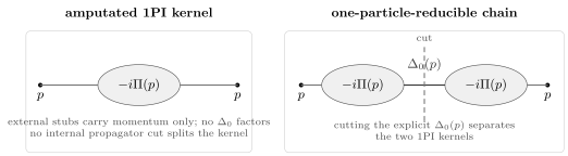
A self-energy insertion is a connected two-point subdiagram that cannot be disconnected by cutting one internal propagator. A chain of two such insertions separated by an ordinary propagator is connected but one-particle reducible.

This distinction is not aesthetic. It prevents overcounting. Once all 1PI self-energy insertions are known, all connected two-point diagrams can be reconstructed by allowing any number of such insertions along a propagator line.

Dyson equation as a geometric series

Let the full amputated 1PI two-point insertion be $-i\Pi(p)$. The connected two-point function is the sum of a free propagator, a free propagator with one self-energy insertion, a free propagator with two self-energy insertions, and so on:

$$\Delta(p)=\Delta_0(p) +\Delta_0(p)[-i\Pi(p)]\Delta_0(p) +\Delta_0(p)[-i\Pi(p)]\Delta_0(p)[-i\Pi(p)]\Delta_0(p) +\cdots.$$

Because translation invariance turns spacetime convolutions into multiplication in momentum space, this is an ordinary geometric series. This step is one of the main benefits of working in momentum space: a chain of kernels becomes multiplication by the same function of $p$. Factoring out $\Delta_0(p)$ gives

$$\Delta(p) =\Delta_0(p) \left[1+[-i\Pi(p)]\Delta_0(p) +([-i\Pi(p)]\Delta_0(p))^2+\cdots\right].$$

Hence

$$\Delta(p)=\frac{\Delta_0(p)}{1+i\Pi(p)\Delta_0(p)}.$$

Substituting $\Delta_0(p)=i/(p^2-m^2+i\epsilon)$ yields

$$\boxed{ \Delta(p)=\frac{i}{p^2-m^2-\Pi(p)+i\epsilon}. }$$

Equivalently, in inverse-propagator form,

$$\boxed{ \Delta(p)^{-1}=\Delta_0(p)^{-1}+i\Pi(p). }$$

The inverse form is often the cleanest statement of Dyson’s equation. The full inverse propagator equals the bare inverse propagator plus the 1PI two-point contribution, with the sign determined by the convention for the insertion. Readers can check the convention by expanding the final answer to first order in $\Pi$; it must reproduce the one-insertion term $\Delta_0(-i\Pi)\Delta_0$.

The exact propagator is a geometric series of free propagators connected by 1PI self-energy insertions. In momentum space this chain sums to $\Delta(p)=i/(p^2-m^2-\Pi(p)+i\epsilon)$.

The same equation can also be written as an integral equation in position space:

$$\Delta(x-y)=\Delta_0(x-y) +\int d^dz\,d^dw\,\Delta_0(x-z)[-i\Pi(z-w)]\Delta(w-y),$$

where $\Pi(z-w)$ is the Fourier transform of $\Pi(p)$. This form emphasizes that the propagating quantum travels freely to a point, experiences an irreducible interaction kernel, and then continues as a full propagating quantum.

First self-energy diagrams in φ⁴ theory

For the interaction

$$\mathcal L_I=-\frac{\lambda}{4!}\phi^4,$$

the one-vertex tadpole correction to the two-point function was found previously as

$$\Delta^{(1)}(x_1-x_2) =-\frac{i\lambda}{2}\int d^dy\,\Delta_0(x_1-y)\Delta_0(y-x_2)\Delta_0(0).$$

Fourier transforming the convolution gives

$$\Delta^{(1)}(p)=\Delta_0(p)\left[-\frac{i\lambda}{2}\Delta_0(0)\right]\Delta_0(p).$$

Therefore the one-loop tadpole contribution to the self-energy is

$$\boxed{ -i\Pi_{\mathrm{tad}}=-\frac{i\lambda}{2}\Delta_0(0) =-\frac{i\lambda}{2}\int\frac{d^dk}{(2\pi)^d}\,\frac{i}{k^2-m^2+i\epsilon}. }$$

This term is independent of the external momentum $p$. It therefore has the same form as a correction to $m^2$. This is a structural statement, not yet a finite numerical prediction: $\Delta_0(0)$ is ultraviolet divergent in the continuum and must be regulated before the phrase “mass correction” becomes quantitative.

At second order, the first momentum-dependent self-energy topology in $\phi^4$ theory is the sunset diagram. Removing the two external propagators from the labeled two-point correction gives

$$\boxed{ -i\Pi_{\mathrm{sun}}(p) =\frac{(-i\lambda)^2}{6} \int\frac{d^dk}{(2\pi)^d}\frac{d^dq}{(2\pi)^d} \frac{i}{k^2-m^2+i\epsilon} \frac{i}{q^2-m^2+i\epsilon} \frac{i}{(p-k-q)^2-m^2+i\epsilon}. }$$

The factor $1/6$ is the same symmetry factor that appears in the two-point sunset correction. The difference is only that the external propagators have been amputated, because $\Pi$ is an insertion kernel.

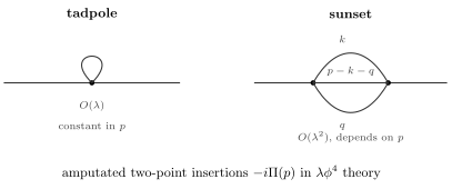
The tadpole is the first self-energy diagram in $\phi^4$ theory and is independent of external momentum. The sunset appears at order $\lambda^2$ and carries nontrivial dependence on $p$ through the three internal propagators.

The ultraviolet behavior of these integrals is not a side issue. A local quantum field has fluctuations at arbitrarily short distances, so loop momenta can become arbitrarily large. In this page we use the diagrams formally to understand organization. Later, power counting and renormalization will explain how the divergent local pieces are absorbed into the parameters of the Lagrangian.

The oscillator viewpoint

A useful way to remember what an interacting propagator means is to write a spectral sum. This is also a good guardrail against overinterpreting individual diagrams: the exact propagator knows about exact energy eigenstates, while self-energy diagrams are a perturbative way of reconstructing their effect. In one time dimension, define the vacuum-subtracted Hermitian operator

$$\widehat\phi=\phi-\langle\Omega|\phi|\Omega\rangle.$$

For exact energy eigenstates $|n\rangle$ of the full Hamiltonian, the connected correlator is

$$\Delta(t)=\langle\Omega|T\widehat\phi(t)\widehat\phi(0)|\Omega\rangle =\sum_{n\ne\Omega} |\langle\Omega|\widehat\phi(0)|n\rangle|^2 \left[\theta(t)e^{-i(E_n-E_\Omega)t}+\theta(-t)e^{i(E_n-E_\Omega)t}\right].$$

Fourier transforming gives

$$\Delta(\omega)= \sum_{n\ne\Omega} |\langle\Omega|\widehat\phi(0)|n\rangle|^2 \left[ \frac{i}{\omega-(E_n-E_\Omega)+i\epsilon} - \frac{i}{\omega+(E_n-E_\Omega)-i\epsilon} \right].$$

For a free oscillator, only one intermediate state contributes to $\phi|0\rangle$, so the propagator has one pair of poles. In an interacting theory, $\phi|\Omega\rangle$ can overlap with many exact states. The self-energy is the perturbative mechanism by which those additional virtual processes deform the simple free pole structure.

In relativistic QFT the same idea is enriched by momentum and multiparticle continua. A stable one-particle state gives an isolated pole. In infinite spatial volume, multiparticle continua give branch cuts; at finite volume they appear instead as a discrete tower of poles that coalesces into a cut as the volume tends to infinity. The Dyson equation does not by itself prove this analytic structure, but it is the perturbative doorway into it.

Constant self-energy as a check

Suppose, as a toy model, that the self-energy is momentum independent:

$$\Pi(p)=\delta m^2.$$

Then Dyson’s equation gives

$$\Delta(p)=\frac{i}{p^2-m^2-\delta m^2+i\epsilon} =\frac{i}{p^2-m_{\mathrm{eff}}^2+i\epsilon},$$

where

$$m_{\mathrm{eff}}^2=m^2+\delta m^2.$$

This is exactly what we expect: a constant two-point insertion has the same effect as a shift of the mass parameter in the quadratic part of the Lagrangian. The tadpole diagram in $\phi^4$ theory has precisely this form before renormalization.

If $\Pi(p)$ depends on momentum, the effect is richer. The pole position is shifted, but the slope of the inverse propagator at the pole is also changed. With the convention used here, the pole residue is the inverse slope,

$$Z=\frac{1}{1-\Pi'(M^2)},$$

not the slope itself.

Summary

The full scalar propagator is not obtained by listing all two-point diagrams one by one. It is obtained more efficiently by separating diagrams into 1PI self-energy insertions and chains made by joining those insertions with free propagators.

With the convention that the amputated 1PI two-point insertion is $-i\Pi(p)$, the exact propagator obeys

$$\Delta(p)=\Delta_0(p)+\Delta_0(p)[-i\Pi(p)]\Delta(p),$$

and therefore

$$\Delta(p)=\frac{i}{p^2-m^2-\Pi(p)+i\epsilon}.$$

The one-loop tadpole in $\phi^4$ theory contributes a momentum-independent self-energy and behaves like a mass correction. The two-loop sunset diagram is the first self-energy diagram in this theory with genuine external-momentum dependence. These corrections are the perturbative origin of dressed particles, shifted poles, residues, multiparticle thresholds, and ultimately renormalized parameters.

Common pitfalls

• The self-energy is not the full correction to the two-point function. It is the amputated 1PI part of the correction.
• A connected two-point diagram can still be one-particle reducible. The Dyson equation uses 1PI insertions precisely to avoid double-counting reducible chains.
• The sign of $\Pi$ depends on convention. Always check whether the insertion is called $i\Pi$, $-i\Pi$, $i\Sigma$, or $\Sigma$.
• A constant self-energy may be absorbed into a mass shift, but a momentum-dependent self-energy also changes the pole residue.
• The bare mass in the Lagrangian and the physical pole mass are not generally the same in an interacting theory.
• Tadpole integrals such as $\Delta_0(0)$ are ultraviolet divergent in continuum QFT. They must be regulated before they can be interpreted quantitatively.

Exercises

Exercise 1

Starting from

$$\Delta(p)=\Delta_0(p)+\Delta_0(p)[-i\Pi(p)]\Delta_0(p)+\Delta_0(p)[-i\Pi(p)]\Delta_0(p)[-i\Pi(p)]\Delta_0(p)+\cdots,$$

show that

$$\Delta(p)=\frac{i}{p^2-m^2-\Pi(p)+i\epsilon}$$

when $\Delta_0(p)=i/(p^2-m^2+i\epsilon)$.

Solution

Factor out $\Delta_0(p)$ on the left:

$$\Delta(p)=\Delta_0(p) \sum_{n=0}^{\infty}\left([-i\Pi(p)]\Delta_0(p)\right)^n.$$

This is a geometric series, so

$$\Delta(p)=\frac{\Delta_0(p)}{1-[-i\Pi(p)]\Delta_0(p)} =\frac{\Delta_0(p)}{1+i\Pi(p)\Delta_0(p)}.$$

Using

$$\Delta_0(p)=\frac{i}{p^2-m^2+i\epsilon},$$

we get

$$1+i\Pi(p)\Delta_0(p) =1+i\Pi(p)\frac{i}{p^2-m^2+i\epsilon} =1-\frac{\Pi(p)}{p^2-m^2+i\epsilon}.$$

Therefore

$$\Delta(p)= \frac{i}{p^2-m^2+i\epsilon} \frac{p^2-m^2+i\epsilon}{p^2-m^2-\Pi(p)+i\epsilon} =\frac{i}{p^2-m^2-\Pi(p)+i\epsilon}.$$

Exercise 2

Use the one-loop tadpole correction

$$\Delta^{(1)}(x_1-x_2) =-\frac{i\lambda}{2}\int d^dy\,\Delta_0(x_1-y)\Delta_0(y-x_2)\Delta_0(0)$$

to identify the corresponding self-energy insertion.

Solution

Fourier transform the two external propagators:

$$\Delta_0(x_1-y)=\int\frac{d^dp}{(2\pi)^d}\,e^{-ip\cdot(x_1-y)}\Delta_0(p),$$ $$\Delta_0(y-x_2)=\int\frac{d^dq}{(2\pi)^d}\,e^{-iq\cdot(y-x_2)}\Delta_0(q).$$

The integral over $y$ gives

$$\int d^dy\,e^{ipy}e^{-iqy}=(2\pi)^d\delta^{(d)}(p-q),$$

so

$$\Delta^{(1)}(p)=\Delta_0(p)\left[-\frac{i\lambda}{2}\Delta_0(0)\right]\Delta_0(p).$$

Comparing with the Dyson form

$$\Delta^{(1)}(p)=\Delta_0(p)[-i\Pi_{\mathrm{tad}}]\Delta_0(p),$$

we find

$$\Pi_{\mathrm{tad}}=\frac{\lambda}{2}\Delta_0(0).$$

Equivalently,

$$-i\Pi_{\mathrm{tad}} =-\frac{i\lambda}{2}\int\frac{d^dk}{(2\pi)^d}\,\frac{i}{k^2-m^2+i\epsilon}.$$

Exercise 3

Assume $\Pi(p)=\delta m^2$ is independent of $p$. Expand the Dyson-resummed propagator to first order in $\delta m^2$ and check that it agrees with a single self-energy insertion.

Solution

The resummed propagator is

$$\Delta(p)=\frac{i}{p^2-m^2-\delta m^2+i\epsilon}.$$

For small $\delta m^2$,

$$\Delta(p) =\frac{i}{p^2-m^2+i\epsilon} \frac{1}{1-\delta m^2/(p^2-m^2+i\epsilon)}.$$

Expanding to first order gives

$$\Delta(p)=\frac{i}{p^2-m^2+i\epsilon} +\frac{i\delta m^2}{(p^2-m^2+i\epsilon)^2}+O((\delta m^2)^2).$$

The one-insertion term is

$$\Delta_0(p)[-i\Pi]\Delta_0(p) =\frac{i}{D}(-i\delta m^2)\frac{i}{D} =\frac{i\delta m^2}{D^2}, \qquad D=p^2-m^2+i\epsilon.$$

This agrees with the first-order expansion of the resummed result.

Exercise 4

Why is the one-loop tadpole self-energy in $\phi^4$ theory momentum independent, while the sunset self-energy is momentum dependent?

Solution

The tadpole self-energy is obtained after amputating the two external propagators from the one-loop two-point correction. The remaining loop is closed at a single vertex:

$$-i\Pi_{\mathrm{tad}} =-\frac{i\lambda}{2}\int\frac{d^dk}{(2\pi)^d}\,\frac{i}{k^2-m^2+i\epsilon}.$$

There is no path through the loop carrying the external momentum $p$. Momentum conservation at the single vertex is already satisfied by the two amputated external legs, and the closed loop momentum is independent. Hence the result is a constant.

For the sunset graph, after the two external legs are amputated there are two vertices connected by three internal propagators. The external momentum enters at one vertex and leaves at the other. If two loop momenta are $k$ and $q$, the third internal line carries momentum $p-k-q$. Therefore

$$-i\Pi_{\mathrm{sun}}(p) =\frac{(-i\lambda)^2}{6} \int\frac{d^dk}{(2\pi)^d}\frac{d^dq}{(2\pi)^d} \frac{i}{k^2-m^2+i\epsilon} \frac{i}{q^2-m^2+i\epsilon} \frac{i}{(p-k-q)^2-m^2+i\epsilon}.$$

The external momentum appears explicitly, so the sunset contributes nontrivial momentum dependence.

References and further reading

• Sidney Coleman, Lectures of Sidney Coleman on Quantum Field Theory, Chapters 8 and 10, for Wick diagrams, connected diagrams, mass renormalization, and self-energy organization.
• Mark Srednicki, Quantum Field Theory, Sections 13–15, for the exact propagator, loop corrections to the propagator, and the Källén–Lehmann perspective.
• Steven Weinberg, The Quantum Theory of Fields, Volume I, Chapters 10–12, for pole structure, field and mass renormalization, and general renormalization theory.
• Michael E. Peskin and Daniel V. Schroeder, An Introduction to Quantum Field Theory, Sections 7.1–7.2, for the Dyson-resummed propagator and one-particle-irreducible functions.

References

Section titled “References”- Schwartz, Matthew D. Quantum Field Theory and the Standard Model. Cambridge University Press, 2014. DOI: 10.1017/9781139540940. § 18.3, p. 330, constructs the 1PI chain and its geometric-series organization for the fermion propagator.
Further reading
Section titled “Further reading”- Coleman, Sidney. Lectures of Sidney Coleman on Quantum Field Theory. Edited by Bryan Gin-ge Chen, David Derbes, David Griffiths, Brian Hill, Richard Sohn, and Yuan-Sen Ting. World Scientific, 2019. DOI: 10.1142/9371. Chapters 8 and 10 discuss Wick diagrams, connected diagrams, and mass renormalization.
- Peskin, Michael E., and Daniel V. Schroeder. An Introduction to Quantum Field Theory. Addison-Wesley, 1995. Publisher. §§ 7.1–7.2 discuss the full propagator and its corrections.
- Srednicki, Mark. Quantum Field Theory. Cambridge University Press, 2007. DOI: 10.1017/CBO9780511813917. §§ 13–15 treat the exact propagator and loop corrections.
- Weinberg, Steven. The Quantum Theory of Fields, Volume I: Foundations. Cambridge University Press, 1995. DOI: 10.1017/CBO9781139644167. Chapters 10–12 develop pole structure, field and mass renormalization, and general renormalization theory.