Skip to content

Nonrelativistic Field Operators

The occupation-number language of the previous page is already close to field theory. It labels states by how many particles occupy each one-particle mode. The next step is to stop treating the mode label as an abstract index and package all creation and annihilation operators into position-dependent operators.

For nonrelativistic particles, this step is not forced by Lorentz invariance. It is a gentler fact: ordinary NN-body quantum mechanics can be rewritten as an operator theory on Fock space. The field operator ψ(x)\psi(\mathbf x) annihilates a particle at position x\mathbf x, while ψ(x)\psi^\dagger(\mathbf x) creates one there. Once this is done, the one-body Hamiltonian, the density, and pairwise interactions all become compact operator expressions.

The payoff is large. A many-body Schrödinger equation with a different wavefunction for each particle number becomes one Hilbert-space equation

iddtΨ(t)=HΨ(t)i\frac{d}{dt}|\Psi(t)\rangle=H|\Psi(t)\rangle

on Fock space. Later, relativistic QFT will use the same logic, but with a crucial upgrade: particle number need not be conserved, and antiparticles and relativistic causality will become unavoidable.

From momentum modes to fields in position space

Section titled “From momentum modes to fields in position space”

Start with bosonic annihilation and creation operators apa_{\mathbf p} and apa_{\mathbf p}^\dagger for momentum modes. In a box, the free nonrelativistic Hamiltonian is

H0=pp22mapap.H_0=\sum_{\mathbf p}\frac{\mathbf p^2}{2m}a_{\mathbf p}^\dagger a_{\mathbf p}.

The position-space field is the Fourier transform of these mode operators,

ψ(x)=1Vpeipxap,ψ(x)=1Vpeipxap.\psi(\mathbf x)=\frac{1}{\sqrt V}\sum_{\mathbf p}e^{i\mathbf p\cdot\mathbf x}a_{\mathbf p}, \qquad \psi^\dagger(\mathbf x)=\frac{1}{\sqrt V}\sum_{\mathbf p}e^{-i\mathbf p\cdot\mathbf x}a_{\mathbf p}^\dagger.

The inverse transform is

ap=1VVd3xeipxψ(x),ap=1VVd3xeipxψ(x).a_{\mathbf p}=\frac{1}{\sqrt V}\int_V d^3x\,e^{-i\mathbf p\cdot\mathbf x}\psi(\mathbf x), \qquad a_{\mathbf p}^\dagger=\frac{1}{\sqrt V}\int_V d^3x\,e^{i\mathbf p\cdot\mathbf x}\psi^\dagger(\mathbf x).

The word “field” here should not be mystical. It means that we have an annihilation operator for every point in space, just as apa_{\mathbf p} is an annihilation operator for every momentum mode. The field is operator-valued because creating and annihilating particles changes the state in Hilbert space.

Using the inverse transform in H0H_0 gives the coordinate-space Hamiltonian. Since multiplication by p2\mathbf p^2 in momentum space is the same as acting with 2-\nabla^2 in position space,

H0=12md3xψ(x)ψ(x).H_0=\frac{1}{2m}\int d^3x\,\nabla\psi^\dagger(\mathbf x)\cdot\nabla\psi(\mathbf x).

Integrating by parts, assuming periodic boundary conditions or fields that vanish sufficiently fast at infinity,

H0=d3xψ(x)(22m)ψ(x).H_0=\int d^3x\,\psi^\dagger(\mathbf x)\left(-\frac{\nabla^2}{2m}\right)\psi(\mathbf x).

This is the first example of the second-quantization rule: a one-particle operator is placed between ψ\psi^\dagger and ψ\psi and integrated over space.

The local field algebra follows directly from the mode algebra:

[ψ(x),ψ(y)]=1Vp,qeipxeiqy[ap,aq]=1Vpeip(xy)δV(3)(xy).\begin{aligned} [\psi(\mathbf x),\psi^\dagger(\mathbf y)] &=\frac{1}{V}\sum_{\mathbf p,\mathbf q} e^{i\mathbf p\cdot\mathbf x}e^{-i\mathbf q\cdot\mathbf y} [a_{\mathbf p},a_{\mathbf q}^\dagger] \\ &=\frac{1}{V}\sum_{\mathbf p}e^{i\mathbf p\cdot(\mathbf x-\mathbf y)} \\ &\equiv \delta_V^{(3)}(\mathbf x-\mathbf y). \end{aligned}

Here δV(3)\delta_V^{(3)} is the periodic delta function on the box. In the infinite-volume limit,

1Vpd3p(2π)3,\frac{1}{V}\sum_{\mathbf p}\longrightarrow \int\frac{d^3p}{(2\pi)^3},

and therefore

[ψ(x),ψ(y)]=d3p(2π)3eip(xy)=δ(3)(xy).[\psi(\mathbf x),\psi^\dagger(\mathbf y)] =\int\frac{d^3p}{(2\pi)^3}e^{i\mathbf p\cdot(\mathbf x-\mathbf y)} =\delta^{(3)}(\mathbf x-\mathbf y).

The remaining commutators vanish:

[ψ(x),ψ(y)]=0,[ψ(x),ψ(y)]=0.[\psi(\mathbf x),\psi(\mathbf y)]=0, \qquad [\psi^\dagger(\mathbf x),\psi^\dagger(\mathbf y)]=0.

Strictly speaking, ψ(x)\psi(\mathbf x) is an operator-valued distribution. The honest operator is a smeared field

ψ(f)=d3xf(x)ψ(x),ψ(f)=d3xf(x)ψ(x),\psi(f)=\int d^3x\,f^*(\mathbf x)\psi(\mathbf x), \qquad \psi^\dagger(f)=\int d^3x\,f(\mathbf x)\psi^\dagger(\mathbf x),

with square-integrable test function ff. Then

[ψ(f),ψ(g)]=fg.[\psi(f),\psi^\dagger(g)]=\langle f|g\rangle.

The delta function in the unsmeared commutator is the kernel version of this finite inner product.

These equations already contain the bosonic exchange symmetry. Since two creation fields commute,

ψ(x1)ψ(x2)0=ψ(x2)ψ(x1)0.\psi^\dagger(\mathbf x_1)\psi^\dagger(\mathbf x_2)|0\rangle = \psi^\dagger(\mathbf x_2)\psi^\dagger(\mathbf x_1)|0\rangle.

A two-particle state created this way is automatically symmetric. There is no separate symmetrization step.

The time-dependent Heisenberg field is defined by

ψ(x,t)=eiHtψ(x)eiHt.\psi(\mathbf x,t)=e^{iHt}\psi(\mathbf x)e^{-iHt}.

Its equation of motion is

itψ(x,t)=[ψ(x,t),H].i\partial_t\psi(\mathbf x,t)=[\psi(\mathbf x,t),H].

For the free Hamiltonian,

[ψ(x),H0]=d3y[ψ(x),ψ(y)](y22m)ψ(y)=d3yδ(3)(xy)(y22m)ψ(y)=x22mψ(x).\begin{aligned} [\psi(\mathbf x),H_0] &=\int d^3y\,[\psi(\mathbf x),\psi^\dagger(\mathbf y)] \left(-\frac{\nabla_{\mathbf y}^2}{2m}\right)\psi(\mathbf y) \\ &=\int d^3y\,\delta^{(3)}(\mathbf x-\mathbf y) \left(-\frac{\nabla_{\mathbf y}^2}{2m}\right)\psi(\mathbf y) \\ &=-\frac{\nabla_{\mathbf x}^2}{2m}\psi(\mathbf x). \end{aligned}

Thus

itψ(x,t)=22mψ(x,t).i\partial_t\psi(\mathbf x,t) =-\frac{\nabla^2}{2m}\psi(\mathbf x,t).

This equation looks like the one-particle Schrödinger equation, but its interpretation is different. In ordinary quantum mechanics, a wavefunction is a complex-valued coefficient of a state. Here ψ(x,t)\psi(\mathbf x,t) is an operator-valued distribution. Matrix elements of this operator obey Schrödinger-type equations because the operator creates and destroys particles whose single-particle energy is p2/(2m)\mathbf p^2/(2m).

The distinction is algebraic, not merely notational: the field has the nontrivial commutator [ψ(x),ψ(y)]=δ(3)(xy)[\psi(\mathbf x),\psi^\dagger(\mathbf y)]=\delta^{(3)}(\mathbf x-\mathbf y) and changes particle number. Indeed, because [N,ψ]=ψ[N,\psi]=-\psi,

eiαNψ(x)eiαN=eiαψ(x).e^{i\alpha N}\psi(\mathbf x)e^{-i\alpha N} =e^{-i\alpha}\psi(\mathbf x).

This is the action of the number-symmetry generator on an operator. It should not be confused with the physically irrelevant overall phase of a state vector.

In momentum space,

iddtap(t)=p22map(t),i\frac{d}{dt}a_{\mathbf p}(t)=\frac{\mathbf p^2}{2m}a_{\mathbf p}(t),

so

ap(t)=eip2t/(2m)ap(0),a_{\mathbf p}(t)=e^{-i\mathbf p^2t/(2m)}a_{\mathbf p}(0),

and

ψ(x,t)=1Vpeipxip2t/(2m)ap(0).\psi(\mathbf x,t) =\frac{1}{\sqrt V}\sum_{\mathbf p} e^{i\mathbf p\cdot\mathbf x-i\mathbf p^2t/(2m)}a_{\mathbf p}(0).

This is the operator version of the free Schrödinger wave expansion.

Define the distributional coordinate ket

x1,,xNu=ψ(x1)ψ(xN)0.|\mathbf x_1,\ldots,\mathbf x_N\rangle_u = \psi^\dagger(\mathbf x_1)\cdots\psi^\dagger(\mathbf x_N)|0\rangle.

The subscript uu reminds us that this basis is unnormalized in the same distributional sense that x|\mathbf x\rangle is unnormalized. Because the creation fields commute, the ket is symmetric under permutations of x1,,xN\mathbf x_1,\ldots,\mathbf x_N.

Now commute ψ(x)\psi(\mathbf x) through the product of creation fields:

ψ(x)ψ(x1)ψ(xN)=k=1Nδ(3)(xxk)ψ(x1)ψ(xk)^ψ(xN)+ψ(x1)ψ(xN)ψ(x).\begin{aligned} \psi(\mathbf x) \psi^\dagger(\mathbf x_1)\cdots\psi^\dagger(\mathbf x_N) &= \sum_{k=1}^N \delta^{(3)}(\mathbf x-\mathbf x_k) \psi^\dagger(\mathbf x_1)\cdots \widehat{\psi^\dagger(\mathbf x_k)} \cdots\psi^\dagger(\mathbf x_N) \\ &\quad+ \psi^\dagger(\mathbf x_1)\cdots\psi^\dagger(\mathbf x_N)\psi(\mathbf x). \end{aligned}

The hat means that the factor is omitted. Since ψ(x)0=0\psi(\mathbf x)|0\rangle=0, the last term vanishes on the vacuum. Therefore

ψ(x)x1,,xNu=k=1Nδ(3)(xxk)x1,,x^k,,xNu.\psi(\mathbf x)|\mathbf x_1,\ldots,\mathbf x_N\rangle_u = \sum_{k=1}^N \delta^{(3)}(\mathbf x-\mathbf x_k) |\mathbf x_1,\ldots,\widehat{\mathbf x}_k,\ldots,\mathbf x_N\rangle_u.

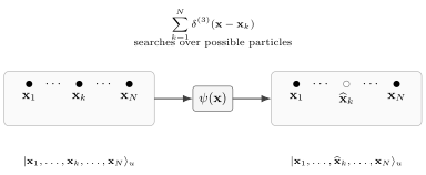
This is the promised local meaning of ψ(x)\psi(\mathbf x): it removes a particle at x\mathbf x, and the delta functions search through the unordered list of particle positions.

A field operator annihilating one particle from a symmetric many-particle state

The annihilation field ψ(x)\psi(\mathbf x) acts on an NN-particle coordinate ket by summing over all possible particles it could remove. Each term carries δ(3)(xxk)\delta^{(3)}(\mathbf x-\mathbf x_k) and leaves an (N1)(N-1)-particle ket with xk\mathbf x_k omitted.

A normalized NN-boson wavefunction ΨN\Psi_N can be embedded into Fock space by

ΨN=1N!d3x1d3xNΨN(x1,,xN)ψ(x1)ψ(xN)0,|\Psi_N\rangle = \frac{1}{\sqrt{N!}}\int d^3x_1\cdots d^3x_N\, \Psi_N(\mathbf x_1,\ldots,\mathbf x_N) \psi^\dagger(\mathbf x_1)\cdots\psi^\dagger(\mathbf x_N)|0\rangle,

with symmetric ΨN\Psi_N and

d3x1d3xNΨN(x1,,xN)2=1.\int d^3x_1\cdots d^3x_N\,|\Psi_N(\mathbf x_1,\ldots,\mathbf x_N)|^2=1.

The inverse map recovers the ordinary wavefunction as a vacuum-to-state matrix element:

ΨN(x1,,xN)=1N!0ψ(xN)ψ(x1)ΨN.\Psi_N(\mathbf x_1,\ldots,\mathbf x_N) = \frac{1}{\sqrt{N!}} \langle0|\psi(\mathbf x_N)\cdots\psi(\mathbf x_1)|\Psi_N\rangle.

The matrix element contains N!N! equal contractions. Together with the 1/N!1/\sqrt{N!} in the definition of ΨN|\Psi_N\rangle, they produce N!ΨN\sqrt{N!}\,\Psi_N; the inverse prefactor above removes precisely that factor. Thus the operator and wavefunction descriptions contain exactly the same information within a fixed-NN sector.

For such a normalized state,

ψ(x)ΨN=N(N1)!d3x2d3xNΨN(x,x2,,xN)ψ(x2)ψ(xN)0.\psi(\mathbf x)|\Psi_N\rangle = \frac{\sqrt N}{\sqrt{(N-1)!}} \int d^3x_2\cdots d^3x_N\, \Psi_N(\mathbf x,\mathbf x_2,\ldots,\mathbf x_N) \psi^\dagger(\mathbf x_2)\cdots\psi^\dagger(\mathbf x_N)|0\rangle.

The factor N\sqrt N is the same occupation-number square root encountered earlier. It appears because there are NN indistinguishable ways to remove one boson.

The local density operator is

ρ(x)=ψ(x)ψ(x).\rho(\mathbf x)=\psi^\dagger(\mathbf x)\psi(\mathbf x).

Using the annihilation formula above,

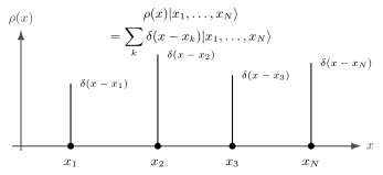
ρ(x)x1,,xNu=k=1Nδ(3)(xxk)x1,,xNu.\rho(\mathbf x)|\mathbf x_1,\ldots,\mathbf x_N\rangle_u = \sum_{k=1}^N\delta^{(3)}(\mathbf x-\mathbf x_k) |\mathbf x_1,\ldots,\mathbf x_N\rangle_u.

So ρ(x)\rho(\mathbf x) measures a spike of density at each particle position.

Density operator represented as delta-function spikes at particle positions

The density operator ρ(x)=ψ(x)ψ(x)\rho(\mathbf x)=\psi^\dagger(\mathbf x)\psi(\mathbf x) acts on a coordinate basis state as kδ(3)(xxk)\sum_k\delta^{(3)}(\mathbf x-\mathbf x_k). In an expectation value, these spikes are smeared by the many-body wavefunction.

The total particle-number operator is

N=d3xρ(x)=d3xψ(x)ψ(x)=papap.N=\int d^3x\,\rho(\mathbf x) =\int d^3x\,\psi^\dagger(\mathbf x)\psi(\mathbf x) =\sum_{\mathbf p}a_{\mathbf p}^\dagger a_{\mathbf p}.

It satisfies

[N,ψ(x)]=ψ(x),[N,ψ(x)]=ψ(x).[N,\psi^\dagger(\mathbf x)]=\psi^\dagger(\mathbf x), \qquad [N,\psi(\mathbf x)]=-\psi(\mathbf x).

Thus ψ\psi^\dagger raises particle number by one, while ψ\psi lowers it by one.

For a normalized NN-particle wavefunction,

ΨNρ(x)ΨN=Nd3x2d3xNΨN(x,x2,,xN)2.\langle \Psi_N|\rho(\mathbf x)|\Psi_N\rangle = N\int d^3x_2\cdots d^3x_N\, |\Psi_N(\mathbf x,\mathbf x_2,\ldots,\mathbf x_N)|^2.

This integrates to NN, not to 11:

d3xρ(x)=N.\int d^3x\,\langle \rho(\mathbf x)\rangle=N.

The density is a particle-counting density. To get the probability density for one randomly selected particle, divide by NN.

Let AA be a one-particle operator with coordinate-space kernel A(x,y)A(\mathbf x,\mathbf y). Acting on a one-particle wavefunction,

(Af)(x)=d3yA(x,y)f(y).(Af)(\mathbf x)=\int d^3y\,A(\mathbf x,\mathbf y)f(\mathbf y).

The corresponding operator on Fock space is

A^=d3xd3yψ(x)A(x,y)ψ(y).\widehat A = \int d^3x\,d^3y\, \psi^\dagger(\mathbf x)A(\mathbf x,\mathbf y)\psi(\mathbf y).

For a local differential operator h(x,i)h(\mathbf x,-i\nabla), this becomes

H^1=d3xψ(x)h(x,i)ψ(x),\widehat H_1 = \int d^3x\, \psi^\dagger(\mathbf x)h(\mathbf x,-i\nabla)\psi(\mathbf x),

where the derivative acts on the field immediately to its right.

The key property is that H^1\widehat H_1 acts on an NN-particle wavefunction as the sum over particles:

H^1k=1Nhk.\widehat H_1 \quad\longleftrightarrow\quad \sum_{k=1}^N h_k.

For example, if

h=22m+U(x),h=-\frac{\nabla^2}{2m}+U(\mathbf x),

then

H^1=d3xψ(x)(22m+U(x))ψ(x)\widehat H_1= \int d^3x\,\psi^\dagger(\mathbf x) \left(-\frac{\nabla^2}{2m}+U(\mathbf x)\right) \psi(\mathbf x)

is the Fock-space version of

k=1N(k22m+U(xk)).\sum_{k=1}^N \left(-\frac{\nabla_k^2}{2m}+U(\mathbf x_k)\right).

The compact field expression is often easier to manipulate than the first-quantized sum, especially once interactions are included.

Now add a symmetric pair potential

V(xy)=V(yx).V(\mathbf x-\mathbf y)=V(\mathbf y-\mathbf x).

In first-quantized notation, the NN-body Hamiltonian is

HN=k=1N(k22m+U(xk))+1i<jNV(xixj).H_N= \sum_{k=1}^N\left(-\frac{\nabla_k^2}{2m}+U(\mathbf x_k)\right) + \sum_{1\le i<j\le N}V(\mathbf x_i-\mathbf x_j).

The field-operator form is

H=d3xψ(x)(22m+U(x))ψ(x)+12d3xd3yψ(x)ψ(y)V(xy)ψ(y)ψ(x).H= \int d^3x\,\psi^\dagger(\mathbf x) \left(-\frac{\nabla^2}{2m}+U(\mathbf x)\right) \psi(\mathbf x) + \frac12\int d^3x\,d^3y\, \psi^\dagger(\mathbf x)\psi^\dagger(\mathbf y) V(\mathbf x-\mathbf y) \psi(\mathbf y)\psi(\mathbf x).

Equivalently,

Hint=12d3xd3y:ρ(x)V(xy)ρ(y):.H_{\mathrm{int}} = \frac12\int d^3x\,d^3y\, :\rho(\mathbf x)V(\mathbf x-\mathbf y)\rho(\mathbf y):.

The colons denote normal ordering: all creation operators are moved to the left of all annihilation operators. This is not just cosmetic. The un-normal-ordered product ρ(x)ρ(y)\rho(\mathbf x)\rho(\mathbf y) includes a self-contraction proportional to δ(3)(xy)ρ(x)\delta^{(3)}(\mathbf x-\mathbf y)\rho(\mathbf x). Normal ordering removes the spurious interaction of a particle with itself. For a contact interaction this distinction is especially important, because the self-term would be proportional to the ill-defined quantity δ(3)(0)\delta^{(3)}(0).

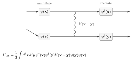
Two-body potential represented by two annihilation fields, a pair potential, and two creation fields

The interaction HintH_{\mathrm{int}} annihilates two particles at x\mathbf x and y\mathbf y, weights the pair by V(xy)V(\mathbf x-\mathbf y), and recreates the two particles. The factor 1/21/2 prevents double-counting the unordered pair (x,y)(\mathbf x,\mathbf y).

Let us verify the action of this term. Acting on an NN-particle coordinate ket, the two annihilation operators remove an ordered pair of particles. The result is

Hintx1,,xNu=12ijV(xixj)x1,,xNu.H_{\mathrm{int}}|\mathbf x_1,\ldots,\mathbf x_N\rangle_u = \frac12\sum_{i\ne j}V(\mathbf x_i-\mathbf x_j) |\mathbf x_1,\ldots,\mathbf x_N\rangle_u.

Since V(xixj)=V(xjxi)V(\mathbf x_i-\mathbf x_j)=V(\mathbf x_j-\mathbf x_i),

12ijV(xixj)=i<jV(xixj).\frac12\sum_{i\ne j}V(\mathbf x_i-\mathbf x_j) = \sum_{i<j}V(\mathbf x_i-\mathbf x_j).

This recovers exactly the first-quantized pair potential. The second-quantized formula is not an approximation. It is the same Hamiltonian written in a language that can act on all particle-number sectors at once.

Recovering the many-body Schrödinger equation

Section titled “Recovering the many-body Schrödinger equation”

Take the full Hamiltonian

H=H1+Hint,H=H_1+H_{\mathrm{int}},

where

H1=d3xψ(x)(22m+U(x))ψ(x),H_1=\int d^3x\,\psi^\dagger(\mathbf x) \left(-\frac{\nabla^2}{2m}+U(\mathbf x)\right)\psi(\mathbf x),

and

Hint=12d3xd3yψ(x)ψ(y)V(xy)ψ(y)ψ(x).H_{\mathrm{int}}= \frac12\int d^3x\,d^3y\, \psi^\dagger(\mathbf x)\psi^\dagger(\mathbf y) V(\mathbf x-\mathbf y) \psi(\mathbf y)\psi(\mathbf x).

For the normalized NN-particle state

ΨN(t)=1N!d3x1d3xNΨN(x1,,xN;t)ψ(x1)ψ(xN)0,|\Psi_N(t)\rangle = \frac{1}{\sqrt{N!}}\int d^3x_1\cdots d^3x_N\, \Psi_N(\mathbf x_1,\ldots,\mathbf x_N;t) \psi^\dagger(\mathbf x_1)\cdots\psi^\dagger(\mathbf x_N)|0\rangle,

the Fock-space Schrödinger equation

iddtΨN(t)=HΨN(t)i\frac{d}{dt}|\Psi_N(t)\rangle=H|\Psi_N(t)\rangle

is equivalent to the ordinary NN-body equation

itΨN=[k=1N(k22m+U(xk))+i<jV(xixj)]ΨN.i\partial_t\Psi_N = \left[ \sum_{k=1}^N \left(-\frac{\nabla_k^2}{2m}+U(\mathbf x_k)\right) + \sum_{i<j}V(\mathbf x_i-\mathbf x_j) \right]\Psi_N.

This equivalence is the main lesson of the page. A field theory can be a rewriting of familiar many-body quantum mechanics. Once that rewriting is in place, it becomes natural to consider Hamiltonians that change particle number, and later relativistic fields whose quanta are particles and antiparticles.

The nonrelativistic field operator is the bridge from many-body quantum mechanics to QFT. It is built by Fourier-transforming the creation and annihilation operators of momentum modes. Its equal-time algebra is local:

[ψ(x),ψ(y)]=δ(3)(xy).[\psi(\mathbf x),\psi^\dagger(\mathbf y)] = \delta^{(3)}(\mathbf x-\mathbf y).

The operator ψ(x)\psi^\dagger(\mathbf x) creates a particle at x\mathbf x, while ψ(x)\psi(\mathbf x) removes one. The density

ρ(x)=ψ(x)ψ(x)\rho(\mathbf x)=\psi^\dagger(\mathbf x)\psi(\mathbf x)

counts particles locally, and N=d3xρ(x)N=\int d^3x\,\rho(\mathbf x) counts particles globally.

The structural dictionary is

k=1Nhkd3xψ(x)hψ(x),\sum_{k=1}^N h_k \quad\longleftrightarrow\quad \int d^3x\,\psi^\dagger(\mathbf x)h\psi(\mathbf x),

and

i<jV(xixj)12d3xd3yψ(x)ψ(y)V(xy)ψ(y)ψ(x).\sum_{i<j}V(\mathbf x_i-\mathbf x_j) \quad\longleftrightarrow\quad \frac12\int d^3x\,d^3y\, \psi^\dagger(\mathbf x)\psi^\dagger(\mathbf y) V(\mathbf x-\mathbf y) \psi(\mathbf y)\psi(\mathbf x).

The notation is heavier at first, but the conceptual payoff is enormous: particles become excitations created and destroyed by fields, and interactions become operator expressions built from local densities. Nothing mystical has happened yet—this is still ordinary many-body quantum mechanics—but the language is now ready for relativistic QFT, where particle number and even the distinction between particles and antiparticles become dynamical.

A field operator is not a many-body wavefunction. The free field equation

itψ=22mψi\partial_t\psi=-\frac{\nabla^2}{2m}\psi

is an operator equation. Wavefunctions are obtained as coefficients of Fock-space states or as matrix elements.

The density ρ(x)\rho(\mathbf x) is not normalized to one. In an NN-particle state,

d3xρ(x)=N.\int d^3x\,\langle \rho(\mathbf x)\rangle=N.

For a probability density of one randomly selected particle, divide by NN.

The expression 12ρVρ\frac12\int \rho V\rho must be normal ordered, or otherwise corrected, if it is meant to represent an interaction between distinct particles. Without this care, it includes a self-interaction term.

Continuum coordinate kets are distributions. Delta functions in formulas involving x1,,xNu|\mathbf x_1,\ldots,\mathbf x_N\rangle_u are not pathologies; they are the many-particle version of xy=δ(3)(xy)\langle\mathbf x|\mathbf y\rangle=\delta^{(3)}(\mathbf x-\mathbf y).

Starting from

ψ(x)=1Vpeipxap,[ap,aq]=δpq,\psi(\mathbf x)=\frac{1}{\sqrt V}\sum_{\mathbf p}e^{i\mathbf p\cdot\mathbf x}a_{\mathbf p}, \qquad [a_{\mathbf p},a_{\mathbf q}^\dagger]=\delta_{\mathbf p\mathbf q},

derive

[ψ(x),ψ(y)]=δV(3)(xy).[\psi(\mathbf x),\psi^\dagger(\mathbf y)]=\delta_V^{(3)}(\mathbf x-\mathbf y).

Then take the infinite-volume limit.

Solution

Using the Fourier expansion,

[ψ(x),ψ(y)]=1Vp,qeipxeiqy[ap,aq]=1Vpeip(xy).\begin{aligned} [\psi(\mathbf x),\psi^\dagger(\mathbf y)] &= \frac{1}{V}\sum_{\mathbf p,\mathbf q} e^{i\mathbf p\cdot\mathbf x}e^{-i\mathbf q\cdot\mathbf y} [a_{\mathbf p},a_{\mathbf q}^\dagger] \\ &= \frac{1}{V}\sum_{\mathbf p}e^{i\mathbf p\cdot(\mathbf x-\mathbf y)}. \end{aligned}

The last expression is the periodic delta function on the box:

δV(3)(xy)=1Vpeip(xy).\delta_V^{(3)}(\mathbf x-\mathbf y) = \frac{1}{V}\sum_{\mathbf p}e^{i\mathbf p\cdot(\mathbf x-\mathbf y)}.

As VV\to\infty,

1Vpd3p(2π)3,\frac{1}{V}\sum_{\mathbf p} \longrightarrow \int\frac{d^3p}{(2\pi)^3},

so

δV(3)(xy)d3p(2π)3eip(xy)=δ(3)(xy).\delta_V^{(3)}(\mathbf x-\mathbf y) \longrightarrow \int\frac{d^3p}{(2\pi)^3}e^{i\mathbf p\cdot(\mathbf x-\mathbf y)} = \delta^{(3)}(\mathbf x-\mathbf y).

Let

x1,,xNu=ψ(x1)ψ(xN)0.|\mathbf x_1,\ldots,\mathbf x_N\rangle_u = \psi^\dagger(\mathbf x_1)\cdots\psi^\dagger(\mathbf x_N)|0\rangle.

Show that

ρ(x)x1,,xNu=k=1Nδ(3)(xxk)x1,,xNu.\rho(\mathbf x)|\mathbf x_1,\ldots,\mathbf x_N\rangle_u = \sum_{k=1}^N\delta^{(3)}(\mathbf x-\mathbf x_k) |\mathbf x_1,\ldots,\mathbf x_N\rangle_u.
Solution

First commute the annihilation field through the product of creation fields:

ψ(x)x1,,xNu=k=1Nδ(3)(xxk)x1,,x^k,,xNu.\psi(\mathbf x)|\mathbf x_1,\ldots,\mathbf x_N\rangle_u = \sum_{k=1}^N \delta^{(3)}(\mathbf x-\mathbf x_k) |\mathbf x_1,\ldots,\widehat{\mathbf x}_k,\ldots,\mathbf x_N\rangle_u.

Then multiply by ψ(x)\psi^\dagger(\mathbf x) on the left:

ρ(x)x1,,xNu=k=1Nδ(3)(xxk)ψ(x)x1,,x^k,,xNu.\rho(\mathbf x)|\mathbf x_1,\ldots,\mathbf x_N\rangle_u = \sum_{k=1}^N \delta^{(3)}(\mathbf x-\mathbf x_k) \psi^\dagger(\mathbf x) |\mathbf x_1,\ldots,\widehat{\mathbf x}_k,\ldots,\mathbf x_N\rangle_u.

Inside the kkth term, the delta function sets x=xk\mathbf x=\mathbf x_k, so the creation operator restores the omitted particle. Thus

ρ(x)x1,,xNu=k=1Nδ(3)(xxk)x1,,xNu.\rho(\mathbf x)|\mathbf x_1,\ldots,\mathbf x_N\rangle_u = \sum_{k=1}^N\delta^{(3)}(\mathbf x-\mathbf x_k) |\mathbf x_1,\ldots,\mathbf x_N\rangle_u.

Show that

Hint=12d3xd3yψ(x)ψ(y)V(xy)ψ(y)ψ(x)H_{\mathrm{int}} = \frac12\int d^3x\,d^3y\, \psi^\dagger(\mathbf x)\psi^\dagger(\mathbf y) V(\mathbf x-\mathbf y) \psi(\mathbf y)\psi(\mathbf x)

acts on an NN-particle coordinate wavefunction as

i<jV(xixj).\sum_{i<j}V(\mathbf x_i-\mathbf x_j).
Solution

The two annihilation fields remove an ordered pair of particles:

ψ(y)ψ(x)x1,,xNu=ijδ(3)(xxi)δ(3)(yxj)x1,,x^i,,x^j,,xNu.\psi(\mathbf y)\psi(\mathbf x)|\mathbf x_1,\ldots,\mathbf x_N\rangle_u = \sum_{i\ne j} \delta^{(3)}(\mathbf x-\mathbf x_i) \delta^{(3)}(\mathbf y-\mathbf x_j) |\mathbf x_1,\ldots,\widehat{\mathbf x}_i,\ldots,\widehat{\mathbf x}_j,\ldots,\mathbf x_N\rangle_u.

The creation fields ψ(x)ψ(y)\psi^\dagger(\mathbf x)\psi^\dagger(\mathbf y) restore the two removed particles. The integrals over x\mathbf x and y\mathbf y evaluate the potential at the removed positions:

Hintx1,,xNu=12ijV(xixj)x1,,xNu.H_{\mathrm{int}}|\mathbf x_1,\ldots,\mathbf x_N\rangle_u = \frac12\sum_{i\ne j}V(\mathbf x_i-\mathbf x_j) |\mathbf x_1,\ldots,\mathbf x_N\rangle_u.

Since VV is symmetric,

12ijV(xixj)=i<jV(xixj).\frac12\sum_{i\ne j}V(\mathbf x_i-\mathbf x_j) = \sum_{i<j}V(\mathbf x_i-\mathbf x_j).

For the free Hamiltonian

H0=d3x12mψ(x)ψ(x),H_0=\int d^3x\,\frac{1}{2m}\nabla\psi^\dagger(\mathbf x)\cdot\nabla\psi(\mathbf x),

show that the density obeys the continuity equation

tρ+j=0,\partial_t\rho+\nabla\cdot\mathbf j=0,

where

j=12mi(ψψ(ψ)ψ).\mathbf j= \frac{1}{2mi}\left(\psi^\dagger\nabla\psi-(\nabla\psi^\dagger)\psi\right).
Solution

The free equations of motion are

itψ=22mψ,itψ=22mψ.i\partial_t\psi=-\frac{\nabla^2}{2m}\psi, \qquad -i\partial_t\psi^\dagger=-\frac{\nabla^2}{2m}\psi^\dagger.

Equivalently,

tψ=i2m2ψ,tψ=i2m2ψ.\partial_t\psi=\frac{i}{2m}\nabla^2\psi, \qquad \partial_t\psi^\dagger=-\frac{i}{2m}\nabla^2\psi^\dagger.

Then

tρ=(tψ)ψ+ψ(tψ)=i2m(2ψ)ψ+i2mψ2ψ=[12mi(ψψ(ψ)ψ)].\begin{aligned} \partial_t\rho &=(\partial_t\psi^\dagger)\psi+\psi^\dagger(\partial_t\psi) \\ &=-\frac{i}{2m}(\nabla^2\psi^\dagger)\psi +\frac{i}{2m}\psi^\dagger\nabla^2\psi \\ &=-\nabla\cdot \left[ \frac{1}{2mi} \left(\psi^\dagger\nabla\psi-(\nabla\psi^\dagger)\psi\right) \right]. \end{aligned}

Therefore

tρ+j=0.\partial_t\rho+\nabla\cdot\mathbf j=0.

The conserved charge associated with this continuity equation is the total particle number N=d3xρ(x)N=\int d^3x\,\rho(\mathbf x).

  • Mark Srednicki, Quantum Field Theory, Section 1, for a compact discussion of rewriting fixed-particle-number nonrelativistic quantum mechanics as a field theory.
  • Sidney Coleman, Lectures of Sidney Coleman on Quantum Field Theory, Chapter 2, for a systematic construction of the many-particle Hilbert space and occupation-number language.
  • Alexander L. Fetter and John D. Walecka, Quantum Theory of Many-Particle Systems, Chapters 1–2, for a many-body perspective on field operators, density operators, and second quantization.
  • A. Zee, Quantum Field Theory in a Nutshell, especially the discussion of field theory without relativity, for physical motivation and condensed-matter connections.