

Confinement and Screening in Two-Dimensional QED
The previous pages developed two complementary viewpoints on two-dimensional fermions. In the gauge-field language, the massless Schwinger model turns the electric field into a massive gauge-invariant excitation. In the bosonic language, a fermion mass term becomes a sine-Gordon cosine, and solitons carry the fermion number. This page puts those two facts to work on a sharp physical question: what is the force between external charges in one spatial dimension?
In pure QED₂, electric flux has nowhere sideways to spread. A pair of opposite static charges is connected by a constant electric field, so the potential grows linearly with separation. Once dynamical charged matter is present, the vacuum can polarize. On the infinite line, massless fermions screen every external charge. In the zero-theta vacuum with positive fermion mass, integer probe charges can be screened by dynamical particles, while fractional probes retain a string tension. The small- and large-mass limits below show how that tension depends on the dynamics. Other exterior flux sectors require the vacuum-energy comparison stated later on this page.
Required background. The Schwinger model and gauge-invariant correlators supplies the exact massless polarization tensor and Schwinger mass. Bosonization and sine-Gordon–Thirring duality supplies the current dictionary, cosine mass perturbation, and soliton charge used below.
Helpful background. The canonical Schwinger-model treatment gives the same mass and probe response with the coupling placed in the covariant derivative; its gauge field and probe charge are and in the notation below.
QED₂ regimes from Gauss’ law
Section titled “QED₂ regimes from Gauss’ law”Two-dimensional normalization. We keep the normalization used in the Schwinger-model page. A unit-charge Dirac fermion is coupled through
The gauge coupling sits in the Maxwell term,
The Lorentzian current and Gauss-law formulas below use the site’s -dimensional extension with .
In real time, with , the electric-field energy density is
External charges are measured in units of the dynamical fermion charge. With one massless Dirac fermion, the Schwinger mass is
The same one-dimensional Gauss law leads to different long-distance behavior depending on which charged degrees of freedom are dynamical.
| Theory | Long-distance potential between and | Physical reason |
|---|---|---|
| Pure QED₂ | flux cannot spread sideways | |
| Massless Schwinger model | saturates | continuous vacuum polarization screens any |
| Massive unit-charge matter, integer | string breaks at large | dynamical particles can screen the endpoint charges |
| Massive unit-charge matter, fractional | residual linear term | only the nearest integer charge can be screened |
This table is the best way to read the page. “Confinement” and “screening” are not labels for a theory in isolation; they are statements about the available dynamical charges and the probe charge being tested.
Pure QED₂ and the linear potential
Section titled “Pure QED₂ and the linear potential”Start with pure electrodynamics in one spatial dimension, coupled to an external static charge density. The real-time action may be written schematically as
Gauss’ law is
For a charge at and a charge at ,
Assume the electric field vanishes outside the interval. Integrating Gauss’ law gives
and
Therefore the energy is
Thus
The coefficient is a one-dimensional string tension. This is a kind of confinement, but it is simpler than the confinement problem in non-Abelian gauge theory. The field is not squeezed into a flux tube by nonlinear dynamics. In one spatial dimension, the “tube” is the whole interval between the charges.
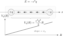
Pure QED₂ has a linear static potential because electric flux cannot spread transversely. Gauss’ law gives a constant electric field between the external charges and zero field outside.
The same result follows from the static propagator. In pure QED₂, the Coulomb kernel is
The interaction energy of opposite charges is
Using
we again obtain
The Fourier form is useful because dynamical fermions modify the kernel directly.
Schwinger screening by massless fermions
Section titled “Schwinger screening by massless fermions”Now include one massless dynamical Dirac fermion. The exact quadratic part of the fermion determinant is transverse:
where
Combining this with the Maxwell term gives
up to gauge-fixing terms in the longitudinal sector. The transverse gauge-field propagator is therefore
For static external charges, this replaces the pure Coulomb kernel by
Thus
The elementary integral
gives
This convention subtracts the coincident configuration, so . The nonzero plateau at is twice the finite energy of the separated screening clouds; only differences in and its derivative are force observables.
At short distance,
so the charges initially see the unscreened one-dimensional Coulomb field. At long distance,
so the potential saturates. The massless fermion has screened the external charge.
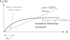
The massless fermion determinant changes the static kernel from to . The linear potential is replaced by a potential that saturates beyond the screening length .
The physics is not subtle, but it is easy to say it imprecisely. The Schwinger mass is not a Proca mass inserted by hand. A local term is not gauge invariant. The determinant instead produces the transverse structure , equivalently a nonlocal gauge-invariant term of the form
Because there is only one gauge-invariant field-strength component in two dimensions, this is enough to make the electric field propagate as a massive scalar.
Bosonized view of screening
Section titled “Bosonized view of screening”Bosonization gives a more local picture of the same screening. Use the convention
For a static configuration,
Let the external charge background be encoded by a step function
so that
Gauss’ law becomes
Choosing the integration constant so that the field vanishes at infinity,
For massless fermions, after discarding the source-independent endpoint self-energy, the static bosonized bulk Hamiltonian in the normalization fixed above is
For the bosonized action, elimination of the electric field on the line, and the resulting scalar mass gap, see Tong 2018, § 7.5.6, pp. 379–380, Eq. (7.70) and the following discussion (PDF).
Inside the interval between the charges, the electric energy is minimized by
Outside the interval, it is minimized by
The static Euler–Lagrange equation is
For , the solution that matches exponentially decaying fields outside the interval is
Consequently, the electric field inside the interval is
For , this field is negative, as required by the earlier Gauss-law orientation. When , it approaches throughout the short interval. For well-separated probes, , it is exponentially small far from the endpoints, and the energy approaches the finite screening-cloud plateau. The figure compares this continuous bulk response with the approximately integer shifts available in the heavy-matter limit.
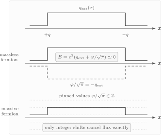
For well-separated massless probes, cancels the bulk electric field continuously. In the leading heavy-matter picture at , , where is the nearest integer to , leaving . The representative case has and . Profiles and boundary-layer widths are schematic and not to scale. At finite fermion mass, the electric quadratic term shifts the minima of the complete potential away from bare cosine minima.
The same statement can be phrased as charge polarization. The dynamical charge density is
For well-separated probes, , the jump of near supplies a charge
which screens the external charge . Near , the opposite jump screens the charge . For massless fermions, need not be an integer. The bosonic field is continuous-valued, and the vacuum can produce arbitrarily soft charge density.
Massive matter and the charge lattice
Section titled “Massive matter and the charge lattice”A fermion mass changes the story qualitatively. The Lorentzian convention is , while Wick rotation gives . With the operator normalization fixed on the preceding page,
where depends on the UV normalization of the fermion mass operator. Up to a field-independent constant, the potential is , whose minima are at
The orientation fixed above assigns an increasing kink positive charge. The integer label is not decorative: it is the charge lattice. A shift
carries total charge
These are minima of the cosine term. The full static potential in a region of constant is
Its stationary points obey
For a fractional probe, an exact cosine minimum generally does not satisfy this equation. The approximately pinned picture requires the cosine term to dominate. The current integral still assigns one unit of charge to a field change ; this does not assert a static soliton joining degenerate vacua of the complete gauged potential.
Thus a massive dynamical fermion can screen an external charge by creating a finite number of particles only when the external charge lies in the integer charge lattice. If
then the external string can break by producing units of dynamical charge near each endpoint. The potential no longer grows indefinitely; at sufficiently large separation, it is energetically cheaper to create particles than to maintain the electric string.
If instead
then pair creation can screen the integer part but cannot screen the fractional part . In a heavy-matter cartoon, the long-distance potential behaves as
where is chosen in the fundamental interval . The additive constant depends on the microscopic mass and binding energy of the screening particles, but the key point is universal: only the fractional unscreened charge contributes to the asymptotic string tension.
Equivalently,
In the heavy-matter limit this periodic tension is approximately
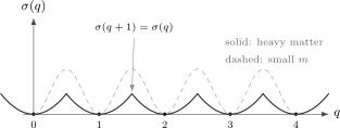
Massive unit-charge matter screens only the integer part of an external charge. In the heavy-matter limit, the residual string tension is approximately quadratic in the distance from the nearest integer charge.
The phrase “integer charges are screened” should always be read in these units: integer means integer multiple of the dynamical matter charge. There is no contradiction with allowing the external probe charge to be any real number. A probe is an external source; dynamical particles live in a quantized charge lattice.
Screening versus string breaking
Section titled “Screening versus string breaking”It is useful to separate two mechanisms that are sometimes lumped together.
In the massless Schwinger model, screening is a linear-response effect. The bosonized field shifts continuously so that the bulk electric field is canceled. No finite pair-creation threshold needs to be crossed, and every external charge is screened.
With massive dynamical matter, screening an endpoint requires creating real charged particles or solitons. The potential may look linear over a long intermediate range, and it flattens only when the energy stored in the electric string is large enough to pay the rest energy of the screening particles. Fractional probe charges cannot be fully screened by integer-charge matter, so a residual string tension remains.
This distinction will reappear in higher-dimensional gauge theory: a Wilson loop can show an area law over an intermediate range even when sufficiently light dynamical matter eventually breaks the string.
Small fermion mass and theta-angle language
Section titled “Small fermion mass and theta-angle language”The massive theory also has a useful theta-angle interpretation. A background electric field in QED₂ is closely related to a theta angle because
shifts the preferred electric flux sector. Inserting a pair of external charges creates a region between them where the effective theta angle is shifted by
Therefore the string tension can be read as a difference of vacuum energy densities:
More precisely, this is the bulk energy-density difference of the flux branch between the probes and the exterior branch. If it is negative, the chosen exterior is metastable and the interval tends to expand; at the stable vacuum used below, the leading result is nonnegative.
For one exactly massless fermion, can be removed by a chiral rotation, and the vacuum energy is independent of . Hence
in the massless Schwinger model.
For a small fermion mass, write . The leading vacuum energy is
At this gives the characteristic periodic form
The numerical value assigned to depends on the normalization convention for , while the product and the periodic dependence are physical. The tension vanishes for integer , is periodic under , and disappears as .
This formula and the heavy-matter formula are not contradictory. They describe different regimes. Heavy matter gives a nearly classical electric string with rare string breaking. Light matter gives a bosonized vacuum energy that is strongly reshaped by the fermion condensate. Both remember the same charge lattice.
Why two dimensions are special
Section titled “Why two dimensions are special”The static Coulomb kernel in spatial dimensions solves
Its large-distance behavior, up to additive constants, is
For opposite charges the interaction energy is proportional to , so the case relevant for QED₂ is extreme: the unscreened potential grows linearly before any non-Abelian dynamics or flux-tube formation has been invoked.
By contrast, in four-dimensional QED the vacuum polarization of light charged particles changes the Coulomb law only logarithmically at short distances. In a one-loop convention with one Dirac fermion,
within perturbation theory. That is screening in the renormalization-group sense, but it is weak compared with Schwinger screening. In QED₂, the gauge coupling has dimension one and the massless fermion determinant generates the finite screening length .
The moral is not that low-dimensional physics is a toy version of higher-dimensional physics. The moral is sharper: changing the number of dimensions changes what electric flux can do.
Summary
Section titled “Summary”Pure QED₂ confines external charges linearly because Gauss’ law forces a constant electric field between them. With our normalization,
Massless dynamical fermions produce the Schwinger mass
so the static kernel becomes and the potential saturates:
Bosonization makes the screening mechanism local: the massless scalar field shifts to cancel the bulk external electric background. A fermion mass adds a periodic cosine contribution to the full potential. Approximately integer bulk shifts describe the heavy-matter limit; the vacuum-energy difference determines the tension more generally. In the zero-theta regime considered here, integer probe charges can be screened by dynamical particles, while fractional charges retain a string tension.
Common pitfalls
Section titled “Common pitfalls”Calling every linear potential “confinement” in the same sense. Pure QED₂ has a linear potential because flux cannot spread in one spatial dimension. Four-dimensional non-Abelian confinement is a much deeper dynamical statement.
Calling the Schwinger mass a Proca mass. A Proca term breaks gauge invariance. The Schwinger mass arises from a transverse, gauge-invariant polarization tensor.
Forgetting the charge lattice. External probe charges can be arbitrary real numbers. Dynamical screening particles have quantized charges. Massive matter screens only the integer part of the probe charge.
Confusing massless screening with pair creation threshold. Massive string breaking requires paying particle rest energy. Massless Schwinger screening is a collective polarization effect and occurs for every external charge.
Interpreting the screened plateau as a residual force. The potential approaches a nonzero constant because each separated probe carries a finite screening-cloud energy. The signed force on increasing separation is for ; it is attractive and vanishes exponentially.
Treating every theta branch as a stable vacuum. The difference is the bulk energy density stored between the probes. A negative value signals decay of a metastable exterior branch rather than a negative stable string tension.
Exercises
Section titled “Exercises”Exercise 1: Linear confinement from Gauss’ law
Section titled “Exercise 1: Linear confinement from Gauss’ law”Use Gauss’ law to derive the pure QED₂ potential between external charges and separated by .
Solution
Gauss’ law is
Take for . Crossing decreases by , so
Crossing increases by , so again for . The electric energy is therefore
Thus
Exercise 2: The screened Fourier kernel
Section titled “Exercise 2: The screened Fourier kernel”Evaluate
for .
Solution
Use the standard Fourier transform
At , this gives
Therefore
Taking and multiplying by gives the screened Schwinger potential.
Exercise 3: Bosonized cancellation of the electric field
Section titled “Exercise 3: Bosonized cancellation of the electric field”Assume the bosonized current is
For the external background
show that the electric field can be written as
up to an integration constant. Explain why a massless bosonized field can screen any in the bulk.
Solution
The total charge density is
Gauss’ law gives
Integrating over ,
If the electric field vanishes at spatial infinity and is chosen to vanish there, then , giving
In the massless theory the static energy contains
but no cosine potential pinning to discrete values. Inside the interval, the field can choose
for any real in the well-separated limit, making the electric field exponentially small far from the endpoints. At finite , the exact profile above retains exponentially overlapping screening layers. Their energy approaches the finite plateau as .
Exercise 4: Residual tension on the charge lattice
Section titled “Exercise 4: Residual tension on the charge lattice”Suppose massive dynamical particles have unit charge. In the heavy-matter limit, argue that an external charge
has asymptotic string tension
Solution
A dynamical particle can screen charge only in integer units. If the external charge is , pair creation can supply charge near the positive external source and charge near the negative external source. This removes the integer part of the electric flux.
The residual unscreened charge is . In one spatial dimension, pure electric flux from charge has tension
The creation of the screening particles adds an -independent energy cost of order , plus binding corrections. At asymptotically large , the coefficient of the term linear in is therefore
The formula is periodic under and vanishes for integer external charge.
Exercise 5: String tension from theta dependence
Section titled “Exercise 5: String tension from theta dependence”Assume that for small fermion mass the vacuum energy density has the leading theta dependence
with . Show that the string tension for a probe charge at is proportional to .
Solution
The external charge shifts the theta angle in the region between the probes by
Therefore
Using the assumed energy density,
Thus
This vanishes for all integer , is periodic under , and goes to zero in the massless limit.
References
Section titled “References”- Tong, David. Gauge Theory. University of Cambridge lecture notes, 2018, § 7.5.6. Official notes. Open PDF: Chapter 7.
Further reading
Section titled “Further reading”- C. Adam, “Charge screening and confinement in the massive Schwinger model,” Physics Letters B 394 (1997), 161–164.
- S. Coleman, “More about the massive Schwinger model,” Annals of Physics 101 (1976), 239–267.
- S. Coleman, Aspects of Symmetry: Selected Erice Lectures (Cambridge University Press, 1985).
- S. Coleman, R. Jackiw, and L. Susskind, “Charge shielding and quark confinement in the massive Schwinger model,” Annals of Physics 93 (1975), 267–275.
- A. M. Polyakov, Gauge Fields and Strings (Harwood Academic Publishers, 1987).
- J. Schwinger, “Gauge invariance and mass. II,” Physical Review 128 (1962), 2425–2429.
- A. Zee, Quantum Field Theory in a Nutshell, 2nd ed. (Princeton University Press, 2010).
- J. Zinn-Justin, Quantum Field Theory and Critical Phenomena, 5th ed. (Oxford University Press, 2021).