

Wilsonian RG and Operator Mixing
The previous page treated the operator product expansion as a local short-distance statement. When two operators approach each other, their product admits an asymptotic expansion in local operators under the stated conditions. This page applies that organization to renormalization-group flow.
The Wilsonian construction is conceptually simple. A theory with ultraviolet cutoff contains field modes with momenta . At a lower resolution , we integrate out the modes in the shell . The exact effective action retains their full momentum-dependent effects. When a local expansion is controlled, those effects can be organized in a larger operator basis:
Here is a reference fixed-point action, are local operators, are their scaling dimensions at the reference point, and are dimensionless couplings. The Wilsonian RG is the differential equation that tells us how the infinite vector changes when the cutoff changes.
This form assumes a basis of scaling operators. In a generic operator basis, the linear flow is a matrix and must be diagonalized. Wilsonian coarse graining and theory space distinguishes exact blocking from a local truncation. Anomalous dimensions and coefficient evolution supply the operator/coefficient duality used in the matrix calculation below.
The key lesson is that renormalization is operator mixing under changes of resolution. Even if the microscopic action contains only one interaction, integrating out a shell generates every operator allowed by the symmetries. Relevant operators grow in the infrared, irrelevant operators are suppressed, and marginal operators require loop calculations. The OPE supplies the local algebra that determines which operators are generated.
Integrating out a momentum shell
Section titled “Integrating out a momentum shell”RG time and flow direction. The shell integrals below are Euclidean. Because the sign of an RG derivative depends on which scale variable increases, we fix the variables explicitly.
We use two related scale variables:
The variable is the running cutoff or probe momentum. Thus increases toward the ultraviolet and increases toward the infrared. We call
the beta function. Written in the infrared coarse-graining time , the same flow is
For four-dimensional scalar theory with , the one-loop convention used in the previous pages is
so lowering the cutoff decreases a positive small :
Split the field into low- and high-momentum parts,
with
The Wilsonian effective action at the lower cutoff is defined by
This definition is exact. A thin shell makes differential flow useful but does not by itself guarantee locality. A derivative expansion also needs small external momenta relative to the removed scales, control of infrared singularities, and an appropriate blocking prescription. In particular, a sharp boundary can produce nonanalytic dependence on external momenta.
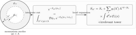
A Wilsonian step integrates out the high-momentum shell . Its exact effect is encoded in ; a local operator expansion is a subsequent approximation under the conditions in the text. The mode split is schematic.
The definition has a semigroup property. If , then integrating first from to and then from to gives the same low-energy functional as integrating directly from to :
This is why the RG is first order in scale. The effective action at the intermediate cutoff carries all information needed for the next step. No memory of exactly how the harder modes were removed is required, except through the couplings already present in .
For low external momenta , a smooth blocking prescription with regular kernels permits a derivative expansion when no infrared singularity obstructs it. With a sharp band, one must separately retain effects of the momentum boundary instead of assuming that every kernel is analytic. Wilson and Kogut keep the general momentum-dependent interactions before introducing their local approximation Wilson and Kogut 1974, Eqs. (4.9), (4.22)–(4.23), pp. 103–106. In four dimensions a local parametrization, when applicable, is
The dots are not a flaw. They are the point. A local effective field theory includes all local operators compatible with the symmetries, organized by their scaling at the resolution of interest.
Scaling and the operator hierarchy
Section titled “Scaling and the operator hierarchy”Suppose the reference fixed point has operators with scaling dimensions . The associated coupling in the action has engineering dimension
It is useful to write the perturbation as
where is dimensionless. Even before loops, changing changes by dimensional analysis. With ,
Equivalently, in infrared time ,
Thus:
| Operator type | Condition | Infrared behavior of |
|---|---|---|
| relevant | grows as is lowered | |
| marginal | decided by loop effects | |
| irrelevant | suppressed as is lowered |
This table is power counting, not a complete RG calculation. Marginal couplings can become marginally relevant or marginally irrelevant. Relevant couplings can be tuned to reach a critical surface. Irrelevant couplings can still be needed for precision matching. But the hierarchy tells us which terms control the infrared without measuring infinitely many parameters.
OPE as the local algebra of RG
Section titled “OPE as the local algebra of RG”The OPE supplies the local rule for what happens when two interaction insertions fall inside the same short-distance shell. Let
Expanding the Euclidean weight gives
When approaches , write and . The OPE gives
The relative coordinate is integrated over the thin shell. If the power of is exactly , the integral is logarithmic:
where
is the area of the unit sphere .
The pure power shown in the OPE assumes scaling operators at a fixed point. Away from a fixed point, the coefficients depend on running couplings and can contain logarithms; the short-distance locality statement remains valid.
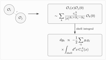
Operator mixing is the Wilsonian consequence of the OPE. When two interaction insertions approach within the eliminated shell, their product is replaced by a sum of local operators. The shell integral shifts the corresponding couplings.
For logarithmic fusion, the quadratic part of the infrared Wilsonian flow has the schematic form
with the understanding that the coefficient depends on the normalization of operators and on how the dimensionless couplings are defined. In ultraviolet beta-function time ,
The sign is easy to forget. In the Euclidean weight, the second-order term appears with a plus sign, because is positive. Re-exponentiating it back into shifts the effective action with the opposite sign. That is why the infrared flow has the minus sign in the quadratic term above.
This displayed quadratic formula is the logarithmic part of the shell calculation. More singular OPE terms produce power-sensitive shifts of relevant couplings such as the mass; less singular terms generate finite or power-suppressed contributions to irrelevant operators. The logarithmic part is singled out because it survives as a scale derivative of a dimensionless coupling.
Example: φ⁴ theory as a Wilsonian flow
Section titled “Example: φ⁴ theory as a Wilsonian flow”Take the four-dimensional scalar theory
at the massless critical point. Define
The previous OPE calculation gives
with
Therefore
In a shell ,
The factor from the second-order expansion of gives
Thus
or
The same step generates higher-field interactions, but the order in depends on the projection being computed. Keep the sharp band above, start from pure interaction, and project onto a constant slow background. Two vertices containing three slow fields and one fast field give at second order
This is a six-field bilocal kernel. Its fast line carries the sum of three external momenta. At constant background that sum is zero, outside the band, so : this term has no local zero-momentum projection. The explicit shell-support constraint is essential Wilson and Kogut 1974, Eqs. (4.22)–(4.23), p. 106.
The first nonzero local six-field coefficient instead comes from the one-loop triangle with three quartic vertices. One can check its sign and coefficient by expanding the fast-mode determinant for a constant background :
Here masses are neglected relative to the shell momenta and controls the background expansion. The same determinant’s quadratic term in reproduces the negative quartic shift already calculated. Thus the four-field coefficient is logarithmic, while this six-field coefficient has mass dimension and vanishes with the shell width. Derivative terms belong to the momentum-dependent calculation. Other blocking prescriptions can assign different power-suppressed coefficients; this result is for the stated sharp-band, constant-background projection.
The figure distinguishes the four- and six-point graphs. Count each vertex’s four incident lines and the external lines left after the fast loop is formed.
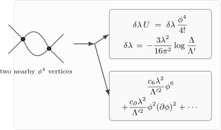
For massless shell propagators with , the bubble contributes at order to , while the triangle contributes at order to the local potential. The order- six-field exchange is bilocal and vanishes at zero external momenta for this sharp band. The graphs are schematic; the coefficients refer to the controlled constant-background expansion above.
This example captures the Wilsonian meaning of perturbative renormalizability. The low-energy theory does contain infinitely many operators, but to predict leading long-distance behavior near the Gaussian fixed point, only the relevant and marginal ones must be controlled. The irrelevant tower is real, but ordered.
Effective actions and low-energy correlators
Section titled “Effective actions and low-energy correlators”The exact Wilsonian effective action preserves normalized low-field correlation functions. Couple the same source to before and after the fast integral, retain the whole effective functional and its normalization, and allow a subsequent field rescaling. For external momenta in the retained band,
where allows for field normalization. There is no additive contact ambiguity for these matched elementary-field sources. A truncated local action only approximates this equality within its momentum and coupling accuracy. Composite insertions require their own matched source operators and may involve contact terms fixed by their subtraction conventions.
For a massive theory with characteristic mass , dimensionless correlators can depend on ratios such as
When
the dependence on is negligible and the dependence on is governed by RG flow. One often writes this schematically as
where the sliding scale is chosen of order the external momenta to avoid large logarithms. This is the practical rule behind RG improvement: do not compute with a coupling defined at a wildly different scale from the process.
Operator mixing as a matrix problem
Section titled “Operator mixing as a matrix problem”So far, coupling mixing came from expanding the action. Composite operators inserted into correlation functions also mix. If is inserted at a point, nearby interaction vertices can fuse with it and produce other operators:
A renormalized operator basis is therefore related to a bare or cutoff basis by a matrix:
The anomalous-dimension matrix is
At fixed bare operator this convention implies
Operator mixing is constrained by symmetries. A scalar even operator cannot mix with a pseudoscalar odd operator. A gauge-invariant operator cannot mix with a gauge-noninvariant observable in physical matrix elements, although gauge-fixed descriptions introduce BRST-exact and equation-of-motion operators. Operators with lower or equal dimension often appear through divergences; higher-dimension operators are generated but power suppressed.
Near a fixed point, the linearized coupling flow is also a matrix problem:
where
Here are engineering dimensions in the chosen basis. The transpose of appears because couplings are dual to operators: the scalar perturbation must be independent of the basis used to represent it. Diagonalizing gives the scaling directions. In a scaling-operator basis its eigenvalues are , and they decide which combinations are relevant, marginal, or irrelevant.
For operators of equal engineering dimension, a scaling combination therefore uses a left eigenvector: gives . A right eigenvector of generally does not supply these coefficients. This follows by differentiating the combination, and is the same duality derived in coefficient evolution. It is compatible with the coupling-column convention in Schwartz 2014, § 23.6, p. 449 after translating which vector the matrix acts on.
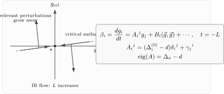
Near a fixed point, the RG is a vector field in coupling space. In infrared time, relevant perturbations leave the critical surface, while irrelevant perturbations within that surface flow toward the fixed point. Quadratic terms are fixed by integrated OPE coefficients.
This is why it is sometimes misleading to say that “the coupling of an operator” runs. Away from a one-dimensional truncation, it is a vector of couplings that runs. The operator basis may rotate as the cutoff changes.
Redundant operators and basis dependence
Section titled “Redundant operators and basis dependence”A Wilsonian effective action is not unique. Field redefinitions change the appearance of the operator basis without changing physical observables. For example, under a local field redefinition
the kinetic term produces operators such as
and the potential produces higher powers of . Some operators can be removed using equations of motion, up to changes in other couplings and contact terms. Such operators are called redundant.
This is not a loophole in the RG. It is basis freedom in the space of local actions. The beta-function components change under a reparametrization of the couplings. Universal statements are invariant: fixed points, critical exponents, the number of relevant directions, and properly defined long-distance observables.
The practical consequence is that one should specify a basis and a subtraction scheme before quoting an anomalous-dimension matrix or a beta-function component. The OPE coefficients in a chosen normalization are meaningful data, but their numerical appearance changes if the operators are rescaled or shifted by other operators.
From cutoff dependence to RG equations
Section titled “From cutoff dependence to RG equations”A physical partition function or correlation function cannot depend on an arbitrary intermediate cutoff. If is computed with the Wilsonian action at scale , then
when all explicit and implicit scale dependence is included. If the only dependence is through couplings and possible field renormalizations, this becomes an RG equation. In a one-coupling truncation,
Here means in the chosen coordinate ; if one switches to , the same equation acquires the corresponding sign change in the beta function. Separating explicit cutoff dependence from implicit dependence through the running coupling gives
For many couplings,
The same logic applied to correlation functions with composite insertions adds anomalous-dimension matrices:
schematically, with each acting on the corresponding operator index. A later page will put this into the standard Callan–Symanzik form.
Summary
Section titled “Summary”The Wilsonian RG is the operation
followed by a local expansion in operators. Its output is not a single renormalized coupling but a full effective action:
Power counting gives the linear hierarchy:
so relevant couplings grow in the infrared, irrelevant couplings shrink, and marginal couplings need loop calculations.
The OPE determines the local quadratic terms in the flow. If
then a logarithmic shell generates a contribution proportional to to the running of . In four-dimensional theory this gives
Composite operators also mix. The mixing matrix and the beta-function vector field are coordinate-dependent descriptions of the same physical fact: changing the resolution changes the local basis in which the theory is described.
Common pitfalls
Section titled “Common pitfalls”Confusing cutoff flow with subtraction-scale flow. With and , the flows differ by a sign.
Keeping only the microscopic operator list. Integrating out modes generates every allowed operator. The reason a finite truncation works is relevance, not absence.
Identifying power divergences with universal beta functions. Power-law pieces are important for matching and naturalness, but logarithmic derivatives of dimensionless marginal couplings are the usual universal perturbative data.
Quoting a mixing matrix without its basis. Total derivatives, equation-of-motion operators, and field redefinitions change the matrix representation of the same physics.
Exercises
Section titled “Exercises”Exercise 1 — Fusion of two distinct interactions
Section titled “Exercise 1 — Fusion of two distinct interactions”Let and suppose
Assume and the sum over in the action is written explicitly, not symmetrized. Find the logarithmic shell contribution to the coefficient of in the effective action after integrating an infrared shell of thickness .
Solution
The second-order term in the Euclidean weight is
if both ordered terms appear in the expansion. For and symmetric OPE coefficients, the two ordered contributions cancel the factor . Thus the logarithmic contribution to the weight is
Using
the weight contains
Since this appears in , it corresponds to the effective-action shift
Therefore the coefficient of shifts by
up to the normalization factors used to make the ‘s dimensionless. If , the factor remains.
Exercise 2 — The Gaussian operator hierarchy
Section titled “Exercise 2 — The Gaussian operator hierarchy”For a scalar field at the Gaussian fixed point in , the engineering dimension is
Classify the operators , , , and as relevant, marginal, or irrelevant by power counting.
Solution
At the Gaussian fixed point in four dimensions,
Thus
so is relevant because .
Next,
so is marginal by engineering dimension.
Also,
so is irrelevant.
Finally,
so is also irrelevant in four dimensions.
Exercise 3 — OPE derivation of the quartic flow
Section titled “Exercise 3 — OPE derivation of the quartic flow”Using
rederive the infrared Wilsonian flow
for .
Solution
First compute the OPE coefficient:
The shell integral in four dimensions is
Since ,
The second-order term in the weight is
Using the OPE in the shell gives
as a contribution to the expansion of . Re-exponentiating it into gives
Therefore
which is the desired flow.
Exercise 4 — Diagonalizing a two-operator mixing matrix
Section titled “Exercise 4 — Diagonalizing a two-operator mixing matrix”Suppose two operators have the same symmetries and the same engineering dimension, and their anomalous-dimension matrix at a fixed point is, with ,
Find the linear combinations with definite anomalous dimensions.
Solution
The eigenvalues of satisfy
Thus
Because , a linear combination evolves with anomalous dimension only when
These are the left eigenvector equations. Convenient choices are
The scaling operators are therefore proportional to
Direct differentiation checks . For example, with , has derivative . The reversed weights , obtained from a right eigenvector of , would instead have derivative and do not scale multiplicatively. Degenerate zero eigenvalues or a non-diagonalizable matrix require a separate analysis; they are excluded by here.
Exercise 5 — The semigroup property of shell flow
Section titled “Exercise 5 — The semigroup property of shell flow”Show that lowering the cutoff in two steps gives the same coupling shift as lowering it in one step, to order , for a single marginal coupling obeying
Solution
For a small interval , solve perturbatively:
Lower first by :
Then lower by :
To order , we may replace by , so
This is exactly the result of one step of size :
The semigroup property is why local shell corrections exponentiate into an RG differential equation.
References
Section titled “References”- Schwartz, Matthew D. Quantum Field Theory and the Standard Model. Cambridge University Press, 2014. DOI.
- Wilson, Kenneth G., and John Kogut. “The Renormalization Group and the Expansion.” Physics Reports 12, no. 2 (1974): 75–199. DOI.
Further reading
Section titled “Further reading”- Cardy, John. Scaling and Renormalization in Statistical Physics. Cambridge: Cambridge University Press, 1996.
- Polchinski, Joseph. “Renormalization and Effective Lagrangians.” Nuclear Physics B 231, no. 2 (1984): 269–295.
- Polyakov, Alexander M. Gauge Fields and Strings. Chur: Harwood Academic Publishers, 1987, Chapter 2.
- Srednicki, Mark. Quantum Field Theory. Cambridge: Cambridge University Press, 2007, Sections 28–29.
- Weinberg, Steven. The Quantum Theory of Fields. Volume II: Modern Applications. Cambridge: Cambridge University Press, 1996, Chapter 18.
- Zinn-Justin, Jean. Quantum Field Theory and Critical Phenomena. 4th ed. Oxford: Clarendon Press, 2002, Chapters 8–13.