

Dimensional Transmutation and Mass Gaps
The previous page ended with the one-loop asymptotically free flow
and therefore
This formula describes dimensional transmutation: instead of specifying a dimensionless coupling at an arbitrary subtraction scale, one may specify an RG-invariant scale such as or . The numerical value of this scale depends on the renormalization scheme; a measurable mass requires additional dynamical information. This lesson derives the scale, explains its continuum-limit meaning, and compares it with the exponential scale in a specified weak-coupling pairing model.
The same idea also explains why perturbation theory can be excellent at short distances while giving no direct perturbative expansion for the masses of bound states. If the generated scale is
then it is non-analytic at . No finite Taylor series in can see it. This is the first warning that mass gaps in asymptotically free theories are nonperturbative, even though their scale is already visible in perturbative RG.
Required background. QED and Yang–Mills Beta Functions fixes the beta-function normalization, derives asymptotic freedom, and supplies the one-loop running used throughout this page.
The RG-invariant scale
Section titled “The RG-invariant scale”Scale variables. Momentum scales such as and denote positive Euclidean magnitudes. On this page
for an asymptotically free coupling. The UV cutoff is written as , where may be a lattice spacing or any short-distance regulator length. When the precise one-loop coefficient is unimportant, we write positive constants as .
Start from the one-loop equation
Integrating gives
where the integration constant has been written as a scale . Solving for gives
Equivalently,
This is the RG-invariant scale. At one loop it is exactly independent of . Beyond one loop its definition is convention-dependent by a multiplicative constant, but the statement that the theory generates a scale is not convention-dependent. Changing the renormalization scheme changes the numerical value assigned to ; it does not change dimensionless physical predictions such as mass ratios.
The all-orders construction makes this precise. In a specified renormalization scheme , define formally
with the finite part of the integration constant included in the definition of the scheme. Differentiating shows . If
then at weak coupling
A redefinition changes the numerical value called by a finite multiplicative factor. It cannot change dimensionless physical predictions such as mass ratios , nor can it remove the essential singularity .
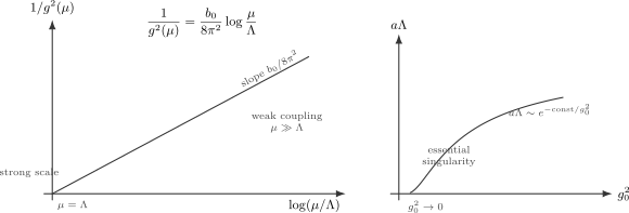
The one-loop asymptotically free flow trades a dimensionless coupling for a dimensionful scale. Its straight inverse-coupling trajectory extrapolates to zero near ; the extrapolation is not a controlled infrared prediction. With a UV cutoff , the RG scale behaves as . Original schematic of the one-loop approximation.
The name “dimensional transmutation” is literal. For this Euclidean cutoff illustration, write the pure Yang–Mills action in terms of a rescaled connection and curvature . With the topological angle fixed to zero, the action is
at the cutoff scale . Classically, is dimensionless and there is no mass parameter. Quantum mechanically, the pair determines
up to scheme-dependent multiplicative factors and higher-loop corrections. To keep finite while taking , one must tune
Thus the continuum limit is not obtained by keeping the bare coupling fixed. It is obtained by approaching the UV fixed point along a trajectory that keeps the physical scale fixed.
The cutoff viewpoint
Section titled “The cutoff viewpoint”The same result can be written in the language of a running coupling measured at momentum below the cutoff. At one loop,
Since , the logarithm is negative. As is lowered, decreases and the coupling grows. The formal scale at which the one-loop denominator vanishes is
The zero of this denominator is a one-loop extrapolation. It cannot establish that the exact coupling diverges. If the flow continues toward strong coupling, perturbation theory fails before that formal pole. More generally, asymptotic freedom alone does not determine the infrared endpoint: higher-order terms can instead produce an infrared fixed point. For example, the beta function with and small is asymptotically free but approaches from below as the scale is lowered. Its leading term alone misses that endpoint.
For ,
is small when the logarithm is sufficiently large. Near the apparent one-loop pole, this formula supplies no controlled value for the coupling. For pure Yang–Mills theory the expected infrared regime is strongly coupled; establishing its spectrum requires nonperturbative physics.
This is why Yang–Mills theory and QCD can be weakly coupled at short distance and strongly coupled at long distance. Short-distance gauge-invariant observables admit a weakly coupled partonic description. Confinement, bound states, and a mass gap concern the infrared and require nonperturbative input.
QED and the opposite flow
Section titled “QED and the opposite flow”It is useful to contrast this with QED. For massless charged matter, the perturbative beta function has the opposite sign,
In momentum variables, the charge grows toward the ultraviolet. In coordinate-space variables, with a distance scale and ,
Therefore
at large in the massless theory. The potential between static charges has the schematic form
If the beta function has no nonzero fixed point, then
so the long-distance charge is screened. In the opposite direction, the one-loop formula develops a UV Landau pole. In the absence of a separate non-Gaussian ultraviolet fixed point, perturbative QED therefore does not furnish the asymptotically free continuum limit available in Yang–Mills theory.
This comparison is conceptually important. Both theories have logarithmic running. But in QED, the massless photon remains in the spectrum and the perturbative flow does not by itself produce a confinement scale. In pure Yang–Mills theory, the coupling grows in the infrared, and the natural expectation is a spectrum of gauge-invariant massive states with masses of order .
What a mass gap means
Section titled “What a mass gap means”A relativistic quantum theory has a mass gap if the vacuum is separated from the rest of the physical spectrum by a positive energy. After choosing a vacuum sector and subtracting its energy, the infinite-volume definition is
This formulation does not assume that the first excitation is a discrete finite-volume level. For a Lorentz-invariant theory, is the smallest invariant mass in the physical Hilbert space. In Euclidean correlation functions, the same statement appears as exponential decay. If is a local gauge-invariant operator with overlap with the lightest state in its channel, then at large Euclidean separation ,
for some power . The smallest such over all nontrivial gauge-invariant channels is the mass gap.
Equivalently, when the asymptotic coefficient is nonzero,
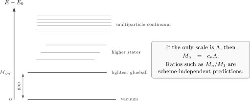
A mass gap is a positive separation between the vacuum and the lightest physical excitation. In pure Yang–Mills theory the expected particles are gauge-invariant glueballs, with masses .
For pure Yang–Mills theory, the expected physical particles are glueballs: gauge-invariant excitations created, for example, by local operators such as . Their masses should have the form
where the are dimensionless numbers. Perturbative RG determines the existence and scaling of , but it does not determine the constants . Those constants are genuinely nonperturbative.
There is a useful distinction here:
but
This distinction keeps the logic honest. Asymptotic freedom strongly suggests where the mass gap should live, but the existence of a mass gap in four-dimensional pure Yang–Mills theory is a nonperturbative statement. The RG argument supplies the only possible scale; it does not by itself prove which gauge-invariant states exist or that the lightest one has strictly positive mass.
In practice one diagnoses a gap by looking for exponential decay in Euclidean correlators of gauge-invariant operators, not by looking for a pole in a gauge-dependent gluon propagator. The latter can be useful in a fixed gauge, but it is not itself the definition of a physical particle. A mass gap and confinement are also logically distinct properties: pure Yang–Mills theory is expected to have both, but the definition of either one does not imply the other in every quantum field theory.
Scaling forms after transmutation
Section titled “Scaling forms after transmutation”Consider a dimensionless physical amplitude depending on a characteristic Euclidean momentum and a coupling defined at a subtraction scale . RG invariance says schematically
For a single-scale observable, the solution may be written in terms of the running coupling at the physical momentum,
For , this becomes a perturbative expansion in
But the same RG equation also says that, after the arbitrary subtraction scale is eliminated, the only dimensionless argument left is
Thus
for a dimensionless observable in a massless one-coupling theory. More generally, if an observable has mass dimension , then
This is the practical content of dimensional transmutation. At finite cutoff, the same dimensionless amplitude can be parametrized as
but after taking the continuum limit along a trajectory of fixed ,
Examples fix the dimensions. A glueball mass has , so . A string tension has , so . A dimensionless short-distance scattering amplitude depends on and becomes expandable in at large momentum.
For QCD with quark masses, additional dimensionless ratios remain:
Here are RG-invariant quark-mass parameters with fixed normalization conventions. Equivalently one can use running masses in a specified scheme, retaining their scale dependence together with that of the coupling. Pure Yang–Mills has no such mass ratios. At fixed gauge group and topological angle, its dimensionless mass ratios are predictions of the theory.
Continuum limits as critical limits
Section titled “Continuum limits as critical limits”The continuum limit of an asymptotically free gauge theory is structurally similar to the continuum limit of a statistical system at a second-order critical point. In both cases a microscopic length is sent to zero while a physical correlation length is held fixed.
In a critical spin system, use the dimensionless reduced temperature with . On a specified side of the transition,
where is measured in lattice units and is a dimensionless, nonuniversal amplitude. The physical correlation length is
so the physical mass scale is
To keep finite as , one tunes .
In asymptotically free Yang–Mills theory, the weak-coupling UV fixed point plays the role of the critical point. The physical scale is
To keep finite as , one tunes .
Compare the exponential bare-coupling tuning with the power-law thermal tuning in the two panels below. Their shared continuum-limit condition does not make the two mechanisms equivalent.
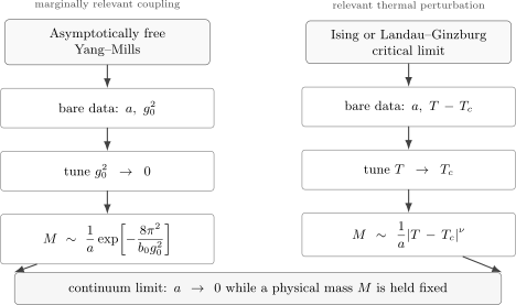
Send the microscopic spacing to zero while tuning a bare parameter so that a physical mass remains finite. The thermal variable is the reduced temperature , and is the dimensionless correlation-length amplitude. The Yang–Mills relation assumes a nonzero mass proportional to its RG scale; one-loop running does not prove that mass gap. Original schematic of exponential versus power-law tuning.
The analogy is not perfect. The Ising temperature perturbation is relevant at the critical point and produces power-law scaling. The Yang–Mills coupling is marginally relevant in the infrared, so the scaling is exponential in . But the logic is the same: a continuum QFT is obtained by making the correlation length large compared with the cutoff.
Essential singularities and invisible perturbative masses
Section titled “Essential singularities and invisible perturbative masses”The exponential dependence
has an essential singularity at . For every nonnegative integer ,
Therefore a mass gap of this type is invisible in ordinary perturbation theory. Any finite perturbative calculation around gives a power series in and logarithms; it cannot produce .
Removing the regulator and probing shorter physical distances are different operations. At fixed , tuning the bare coupling gives
The cutoff cancels: tends to zero as , while the renormalized coupling stays fixed to this order. Regulator removal suppresses cutoff effects; increasing the physical ratio improves the weak-coupling expansion. For a theory with of order , perturbation theory controls sufficiently large
while the mass gap concerns
The RG flow connects the two regimes, but it does not make the infrared perturbative.
A Fermi-surface preview
Section titled “A Fermi-surface preview”A similar exponential scale appears in the Cooper channel. Consider a balanced three-dimensional two-component Fermi liquid with coherent, degenerate partners and . Let be energy relative to the Fermi surface, and retain an instantaneous separable -wave attraction in the sharp energy shell . Write for the constant density of states of one species, per volume and per energy. Thus has units of energy times volume, while
is dimensionless and negative. The subscript distinguishes this channel coupling from the gauge coupling above.
The zero-temperature frequency integral in the normal-state pair bubble gives . Including both sides of the Fermi surface therefore gives
Summing the leading ladders gives . With ,
Here is the formal normal-state pole scale; weak-coupling control is lost before the pole. It does not by itself calculate a gap or a transition temperature. The angular-channel flow has the same normalized form in Shankar 1993, v2, §VI.C, pp. 101–102, Eqs. (383)–(384), PDF; his channel variable has a different phase-space normalization.
To calculate a gap, add the homogeneous zero-temperature BCS mean-field approximation for this reduced-shell model, assuming , , and no competing instability or pair-breaking mismatch. The pairing field mixes particle and hole states through
Diagonalization gives . In the corresponding paired ground state, . The self-consistency condition therefore closes the BCS gap equation:
This is the constant-matrix-element construction of Bardeen, Cooper, and Schrieffer 1957, §II, pp. 1181–1183, Eqs. (2.34)–(2.40) and (2.50), with their positive attraction magnitude replaced by and their by . Their product of the one-spin density of states and interaction matrix element becomes in the per-volume convention here.
The exact saddle has minimum positive quasiparticle energy when the dispersion crosses . The negative BdG branch is its particle–hole partner; the separation of the branches there is . In this model at weak coupling. That prefactor comes from the specified gap integral, not from the normal-state leading logarithm. Follow the conditional step between the two calculations in the figure.
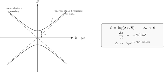
The upper normal-state calculation uses and defines . The dashed arrow requires the stated constant-DOS, sharp-shell, instantaneous BCS mean-field model at zero temperature; its gap obeys at weak coupling. Below, solid curves show the exact normalized BdG branches and dashed lines the normal crossing. The positive minimum is ; the negative branch is a particle–hole partner. Original schematic of the conditional calculation with exact dimensionless dispersion curves, not material data.
The analogy has limits. A Fermi surface is not Lorentz invariant. A nonzero quasiparticle gap is not a proof of phase coherence or a gap to every many-body excitation: a neutral superfluid can retain a gapless phase mode. Mismatch, temperature, or competing channels can also stop the normal-state flow. The shared conclusion is that a logarithm can generate an exponentially small scale; identifying the resulting state requires additional dynamics.
What is and is not proved by the one-loop flow
Section titled “What is and is not proved by the one-loop flow”The leading beta function establishes weak ultraviolet running near the Gaussian fixed point when . Its formal infrared pole indicates the limit of the one-loop extrapolation; it neither excludes an infrared fixed point nor proves confinement, a discrete glueball spectrum, or a positive mass gap.
For pure Yang–Mills theory, the physical expectation is
and lattice gauge theory strongly supports this picture. But from the viewpoint of continuum perturbation theory, the statement remains nonperturbative. This is exactly why dimensional transmutation is so important: it shows how the scale can exist without pretending that weak-coupling diagrams calculate the infrared spectrum.
A good slogan is:
Summary
Section titled “Summary”An asymptotically free theory with
has the one-loop running
The integration constant may be written as the RG-invariant scale
This is dimensional transmutation: the dimensionless coupling is traded for a dimensionful scale.
With a cutoff , the continuum limit of pure Yang–Mills theory is obtained by taking
This resembles the critical continuum limit of a statistical system, where while is held fixed.
A mass gap means a positive separation between the vacuum and the lightest physical state. In pure Yang–Mills theory, the expected spectrum consists of gauge-invariant massive states with
The scale is visible from perturbative RG, but the constants and the existence of the gap are nonperturbative.
Common pitfalls
Section titled “Common pitfalls”Claiming that perturbation theory computes the gap. Perturbation theory determines the high-momentum running and identifies the RG-invariant scale. The gap itself is infrared and nonperturbative.
Treating a one-loop pole as an exact singularity. The pole is a warning that the chosen perturbative variables have failed, not a controlled statement about the exact coupling.
Confusing scheme dependence with physical arbitrariness. A coupling redefinition changes the numerical value assigned to , but physical masses and mass ratios do not depend on that convention. One fixes a scheme for and quotes nonperturbative quantities in that scheme or as dimensionless ratios.
Holding the bare coupling fixed while removing the cutoff. Fixed leaves the correlation length finite in cutoff units. The continuum limit requires so that while in physical units remains fixed.
Equating a mass gap with confinement. They are distinct infrared properties. Pure Yang–Mills theory is expected to possess both, but one-loop asymptotic freedom proves neither.
Assuming every marginal interaction generates a gap. Some marginal interactions are exactly marginal or marginally irrelevant. The sign of the beta function and the interaction channel matter.
Exercises
Section titled “Exercises”Exercise 1: Verify one-loop RG invariance of the transmutation scale
Section titled “Exercise 1: Verify one-loop RG invariance of the transmutation scale”Let
Show that
is independent of at one loop.
Solution
First compute
Using the beta function,
Now differentiate
This gives
Thus is RG invariant at one loop.
Exercise 2: Tune the bare coupling toward the continuum limit
Section titled “Exercise 2: Tune the bare coupling toward the continuum limit”With cutoff , suppose
Solve for in terms of and fixed . What happens as ? Compare at the two cutoffs and , keeping fixed, within the one-loop model.
Solution
Since ,
Multiply by and take the logarithm:
Equivalently,
Therefore
As at fixed , the logarithm diverges and hence
The continuum limit approaches the weak-coupling UV fixed point. In the two-cutoff comparison, set . Then changes from to , but
Thus the renormalized coupling at this fixed physical momentum does not decrease when the cutoff is increased. The comparison tests cutoff cancellation within the one-loop model, not the numerical accuracy of that model at .
Exercise 3: Derive the scaling form after dimensional transmutation
Section titled “Exercise 3: Derive the scaling form after dimensional transmutation”Assume a dimensionless physical observable satisfies the RG equation
Explain why, in a massless one-coupling asymptotically free theory, it can be written as
Solution
The observable is dimensionless, so before solving the RG equation it can only depend on the dimensionless ratio and on the running coupling .
The RG equation says that changing while moving along the RG trajectory leaves unchanged. Therefore the only invariant data on the RG trajectory can appear. For a one-coupling asymptotically free theory, the invariant data are encoded in
at one loop, with higher-loop refinements changing only the precise scheme definition of .
Since is the only external scale and is the only intrinsic scale, dimensional analysis then gives
At , the same statement can be rewritten as a perturbative expansion in .
Exercise 4: Solve the coordinate-space QED flow
Section titled “Exercise 4: Solve the coordinate-space QED flow”In coordinate-space QED, suppose
Solve for with boundary condition . What is the large- behavior?
Solution
Write
Integrating from to gives
Thus
For ,
The charge is screened at long distance. This running alone does not generate a mass gap for the photon.
Exercise 5: Tune a statistical system to its critical limit
Section titled “Exercise 5: Tune a statistical system to its critical limit”Near an Ising critical point, use and a fixed dimensionless amplitude :
The physical correlation length is and the physical mass is . Determine how must scale with if is held fixed while . Translate back to the dimensionful temperature difference.
Solution
The physical mass is
Holding fixed gives
Therefore
As , the temperature must be tuned to . This is the statistical-mechanics analog of tuning in an asymptotically free gauge theory while keeping the physical mass scale fixed.
Exercise 6: Distinguish the Cooper pole from the BCS gap
Section titled “Exercise 6: Distinguish the Cooper pole from the BCS gap”For the dimensionful channel interaction , take a constant one-species density of states and define . The leading flow is
Find the formal pole scale . Under the reduced-shell BCS assumptions in the text, solve the gap integral and compare for . Would replacing by the spin-summed density of states while leaving unchanged preserve the prediction?
Solution
Integrate
This gives
or
Since , the denominator reaches zero at
If the running energy scale is , the formal normal-state pole is
The BCS integral is a separate calculation. With , it gives
Consequently,
Using a spin-summed with unchanged incorrectly doubles . It predicts , an exponentially different scale. A notation change must preserve the product of the correctly counted pair density of states and the matched interaction. Neither normal-state pole alone establishes a paired ground state or phase coherence.
References
Section titled “References”- Bardeen, John, Leon N. Cooper, and J. Robert Schrieffer. “Theory of Superconductivity.” Physical Review 108, no. 5 (1957): 1175–1204. DOI. Open PDF.
- Shankar, Ramamurti. “Renormalization Group Approach to Interacting Fermions.” Reviews of Modern Physics 66 (1994): 129–192. DOI. Cited edition: June 1993 preprint, arXiv:cond-mat/9307009v2. Open PDF.
Further reading
Section titled “Further reading”- Coleman, Sidney, and Erick Weinberg. “Radiative Corrections as the Origin of Spontaneous Symmetry Breaking.” Physical Review D 7, no. 6 (1973): 1888–1910.
- Gell-Mann, Murray, and Francis E. Low. “Quantum Electrodynamics at Small Distances.” Physical Review 95, no. 5 (1954): 1300–1312.
- Gross, David J., and Frank Wilczek. “Ultraviolet Behavior of Non-Abelian Gauge Theories.” Physical Review Letters 30, no. 26 (1973): 1343–1346.
- Politzer, H. David. “Reliable Perturbative Results for Strong Interactions?” Physical Review Letters 30, no. 26 (1973): 1346–1349.
- Polyakov, Alexander M. Gauge Fields and Strings. Chur: Harwood Academic Publishers, 1987, Chapter 2.
- Schwartz, Matthew D. Quantum Field Theory and the Standard Model. Cambridge: Cambridge University Press, 2014, Chapters 23 and 26.
- Srednicki, Mark. Quantum Field Theory. Cambridge: Cambridge University Press, 2007, Sections 28, 73, and 82.
- Weinberg, Steven. The Quantum Theory of Fields. Volume II: Modern Applications. Cambridge: Cambridge University Press, 1996, Chapter 18.
- Wilson, Kenneth G., and John Kogut. “The Renormalization Group and the Expansion.” Physics Reports 12, no. 2 (1974): 75–199.
- Zinn-Justin, Jean. Quantum Field Theory and Critical Phenomena. 4th ed. Oxford: Clarendon Press, 2002.